PivotTable Text Values Alternative with FILTER

This is the third and final post in the PivotTable Text Values Alternative series, where we are discussing alternatives to displaying text values in PivotTables. In the first post, we used Power Query as an alternative. In the second post, we combined multiple text values. In this post, we’ll use the FILTER function as an alternative to PivotTable text values. Let’s get to it.

Objective – PivotTable with Text Values

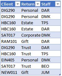
Before we get too far, let’s confirm our goal. We export some data like this:

And we’d like to create a summary report like this:

In our previous posts, we used Power Query as an alternative to using a PivotTable to create this report. This time, we’ll use Excel formulas.

Video – PivotTable Text Values Alternative with FILTER

Narrative

This narrative provides the specific steps to create an alternative to PivotTable text values with the FILTER function. We’ll create the report using the following three steps:

• Report labels with UNIQUE and TRANSPOSE
• Retrieve text values with FILTER
• Join text values with ARRAYTOTEXT

Let’s take these steps one by one.

Note: depending on your version of Excel, you may or may not have access to the functions discussed.

Report Labels

The first step in creating this formula-based report is to create the report labels. These are the row and column headers. As this is Excel, there are several ways to accomplish this.

One option would be to create them manually. To create the row labels, we would copy the entire Client column, and the paste special values in an empty area of the worksheet. Then, we would use the Data > Remove Duplicates command to remove any duplicate values. To create the column labels, we would copy the entire Return column, and then paste special values in an empty area. Then, we would remove duplicates. Then, we could copy and do a paste special transpose. Then, we could move them into place as desired.

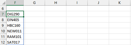
Another option would be to use a formula. To create a list of the unique row labels (no duplicates), we would enter the following formula:

=UNIQUE(Table1[Client])

We hit Enter, and bam:

If we wanted the row labels sorted, we could just wrap the SORT function around the UNIQUE function, like this:

=SORT(UNIQUE(Table1[Client]))

And bam:

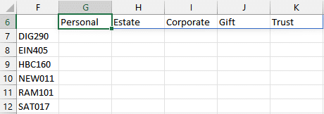
To create the column labels, we would use the UNIQUE function to retrieve a list of the Return column values without duplicates. We want to transpose them from rows to columns, so we wrap the TRANSPOSE function around the UNIQUE function like this:

=TRANSPOSE(UNIQUE(Table1[Return]))

We hit Enter and bam:

With the report labels looking good, it is time to retrieve our text values with the FILTER function.

Retrieve text values with FILTER

We will use the FILTER function to retrieve the text values from the Staff column. We can use the following formula:

=FILTER(Table1[Staff],((Table1[Client]=$F7)*(Table1[Return]=G$6)),"")

Where:

• Table1[Staff] is the column that has the values to return
• ((Table1[Client]=$F7)*(Table1[Return]=G$6)) is the criteria for which values to include
• “” returns an empty string if there are no Staff for any given Client Return

Note: if you’d like to learn more about how to construct the criteria expression, check out this post.

We hit Enter and bam:

We notice that DAR and DMK are both returned. This is because both are assigned to DIG290 Personal. So, we need a way to combine multiple staff values into a single cell. We’ll tackle this final step with ARRAYTOTEXT.

Join text values with ARRAYTOTEXT

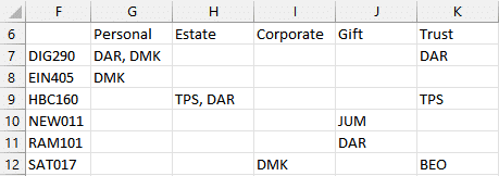
To combine multiple staff values with a comma-space delimiter, we wrap the ARRAYTOTEXT function around the FILTER function, like this:

=ARRAYTOTEXT(FILTER(Table1[Staff],((Table1[Client]=$F7)*(Table1[Return]=G$6)),""))

We hit Enter and bam:

Note: if you wanted to use a delimiter other than a comma-space, you can use TEXTJOIN instead of ARRAYTOTEXT.

Finally, we need to fill the formula down and right. We Copy the formula and Paste it into the other empty cells. Bam:

Note: if you try to fill the formula right by clicking-and-dragging, you’ll probably get unexpected results because the column references will be treated as relative. So, instead of clicking-and-dragging, you’ll want to use Copy/Paste or the Fill > Right command. Also, be sure to use the correct cell reference style, such as $F7 to lock down the column reference and G$6 to lock down the row reference.

With the report labels and values in good shape, we can now apply any desired formatting. This could include bold font for the labels, centering the values, and applying some cell borders:

Yay … we did it!

Conclusion

This is the final post in the series, and I hope it has been helpful.

If you have any alternatives or suggestions, please share by posting a comment below … thanks!

Sample file: