PivotTable Text Values Alternative

One limitation of a traditional PivotTable is that we aren’t able to place text fields into the values layout area. Well, technically we can, but we get a count rather than seeing the text value. In this post, I’ll demonstrate an alternative way to display text values that uses Power Query (instead of a PivotTable). Depending on the type of report you are building, this may be a nice option.

Objective – PivotTable with Text Values

Before we get to the details, let’s review our goal.

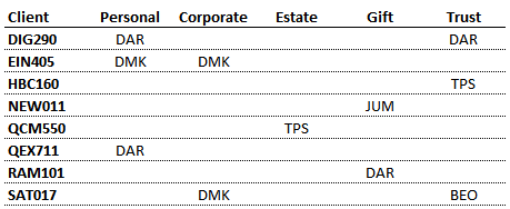
We have exported some data from our system. In this illustration, it is a list of our Clients along with the Staff assigned to do each type of Tax Return. It looks like this:

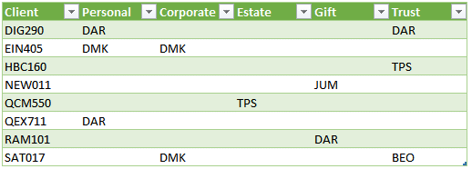
We would like to view it in a way that is easier to read. So, we would like one row per client and one column for each type of tax return. We want to see the assigned staff person in the report. Our goal is to see something like this:

One option that comes to mind is using a PivotTable. So, we use the Insert > PivotTable command. Then, we insert Client into the Rows area, Return into the Columns area, and Staff into the Values area. The resulting PivotTable looks like this:

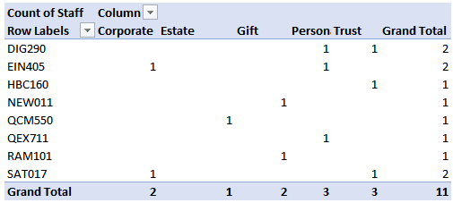
We see the number 1 in the cells where we want to see the staff initials. When we inspect the Values field, we see it has defaulted to Count:

We use the drop-down to see if there are any other Value Field Settings we can use, and we see Min and Max and are filled with hope:

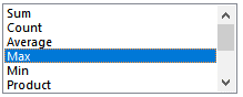
So we try Max and drats … we still do not see the staff initials:

One option here is to stick with a PivotTable, but use the data model and write a measure using the CONCATENATEX DAX function. This is a very cool option that we can use to display text values in a PivotTable and it enables us to join together a string of comma-separated values if needed. Depending on the format of your report and data, that option may be a great fit. More info here.

But, in our case, we only have one staff per client return. So, let’s explore an option that requires only a couple of mouse clicks and uses Power Query instead of a PivotTable.

Walkthrough – Alternative to PivotTable with Text Values

We will create the desired report in three steps:

• Get data into Power Query
• Pivot Transformation
• Load to Excel

Let’s walk through these steps one by one.

Get data into Power Query

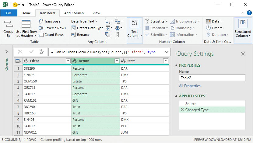
First we need to get the data into Power Query. We can do this by selecting the data table and clicking Data > From Sheet (or depending on your version of Excel, Data > From Table/Range.) The data is pulled into the Power Query editor:

With the data in Power Query, it is time for our next step.

Pivot Transformation

Next, we select the column that contains the values we want to use as our column headers. This is the same field we would put into the Columns layout area of a PivotTable. In our case, we want one column for each value in the Return column, so we select the Return column.

We then click Transform > Pivot Column. In the resulting Pivot Column dialog, we select Staff as the Values Column because it contains the values we want displayed.

Now, the next setting is important and is different than the way a PivotTable works.

Next, we click Advanced options > Maximum (or Minimum) in order to display the text value instead of the default Count:

With a PivotTable, if we use Max or Min on a text value, 0 is displayed. HOWEVER with Power Query, the maximum or minimum text value is displayed (think of it as sorting, and then picking the first or last in the list). We can also use the Don’t Aggregate option when there are not multiple values. Since we only have one unique text value per client return, we are good with Max, Min, or Don’t Aggregate. (If we had multiple staff per client return, Don’t Aggregate will return an error, and so we’ll need to perform additional transformations … and I’ll talk about that in an upcoming post.)

So, we click OK and bam:

Yes … it worked! All that remains is to get the data back into Excel.

Load to Excel

To get the data back into Excel, we click Home > Close & Load To … and we send it to a Table in an existing or new sheet. Bam:

Yay … we did it! And the good news is that if our source data values change, or new client returns are added or assigned, we can simply right-click the green results table and select Refresh. It will instantly update with any changes.

Conclusion

The key to this technique is that we use the Min or Max aggregate function in the Pivot Column transformation. It is important to note because it is different from the way PivotTables work.

Oh … one more thing … using Min/Max in Power Query also works with the Group By transformation.

If you have any thoughts or suggestions, please share by posting a comment below … thanks!

Notes: in addition to using the Pivot Column transformation, Power Query can also Unpivot columns as shown in this post.

Sample File