PivotTable with Multiple Text Values Alternative

If you have tried to insert a text field into the values layout area of a PivotTable, you may have noticed that the text string itself is not displayed. Instead, the count is displayed by default. In this series, we are talking about how to display the desired text values by using Power Query instead of a PivotTable. In the first post, we covered the steps needed when there is only one text value. We will now walk through the steps to join together multiple text values and separate them with a delimiter such as a comma.

Objective – PivotTable with Text Values

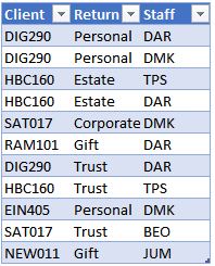
Before we get to the details, let’s confirm our goal here. We’ve exported some data from our system. In this illustration, it is the staff assigned to prepare client tax returns:

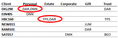
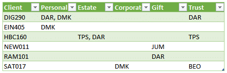
We would like to get it into a format like this, and note that there can be multiple staff assigned:

In our previous post, we attempted to use a PivotTable. We quickly noticed that traditional PivotTables don’t really support the use of text in the values layout area, even when using the Min/Max options. So, we used Power Query as an alternative, and noticed that Min/Max do work with text strings. We could also use the Don’t Aggregate option. In the prior post, we only had a single staff assigned to each return, so Min/Max/Don’t Aggregate all returned the same result.

In this post, we will discuss how to handle the case of multiple text values, how Min/Max/Don’t Aggregate provide different results, and how to join the text values with the delimiter of your choice. Let’s do this thing.

Walkthrough – Power Query Alternative to PivotTable with Text Values

Let’s walk through the following steps:

• Get Data into Power Query
• Perform Transformations
• Return Data to Excel

First things first … we need to get the data into Power Query.

Get Data into Power Query

In this illustration, our data is in an Excel table, but in practice, it could be just about anywhere. We begin by selecting Data > From Sheet. (Or, Data > From Table/Range depending on your version of Excel.)

The data is loaded into the Power Query editor:

With that step complete, we can now perform our transformations.

Perform Transformations

In the previous post, we immediately performed a Pivot Column transformation at this point. That was because we did not have multiple rows for any given client return … in other words, there was only one staff assigned to each client return. However, in this data set, we have client returns with multiple staff assigned. If we were to use the steps shown in the previous post, we would see the following results based on our choice in the Pivot Column dialog (Advanced options):

• Minimum – would return only one of the assigned staff (the first one, alphabetically)
• Maximum – would return one staff (the last one, alphabetically)
• Don’t Aggregate – would return an error (Expression.Error: There were too many elements in the enumeration to complete the operation)

So, our first transformation will NOT be Pivot Column. Instead, our first step is to Group By in order to shrink our table down to one row for each unique combination of Client/Return.

Group By

We start by selecting both the Client and Return columns (as shown above).

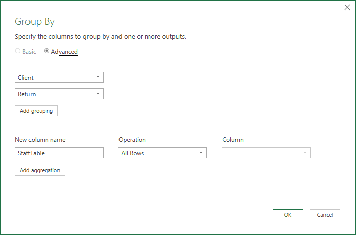
Then we select Transform > Group By. In the resulting Group By dialog, we define a New column name such as StaffTable and set the Operation to All Rows as shown below:

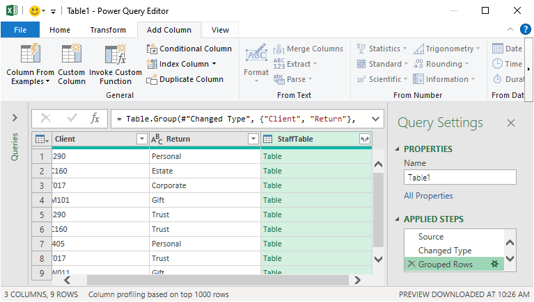
We click OK and see a new column called StaffTable and it looks like it stores a bunch of Tables:

Think of each Table as a little mini-table that contains one row for each staff assigned to that specific Client Return. We can view each mini-table by clicking the empty space in any cell:

We can now move to our next step.

Staff List

The StaffTable column contains a bunch of mini-tables. Instinctively, we understand that in general, a table can include multiple rows and multiple columns. We can verify this by viewing the mini-table in the screenshot above. We confirm there are two rows (one for DAR and one for DMK) and three columns (Client, Return, and Staff).

To accomplish our next step, we need to isolate the Staff column. While a Table can store multiple columns, a List can store a single column. So, our objective is to create a List of staff names for each client return.

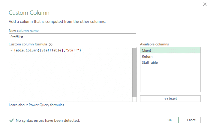
One way to accomplish this is to create a new custom column by clicking Add Column > Custom Column. In the resulting dialog, we give our new column a name, such as StaffList. Then we use the Table.Column function to pull the “Staff” column out of the [StaffTable] table. The formula is shown below:

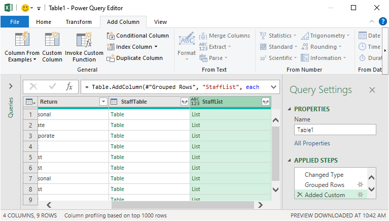
We hit OK, and we see a new column called StaffList that contains a bunch of Lists:

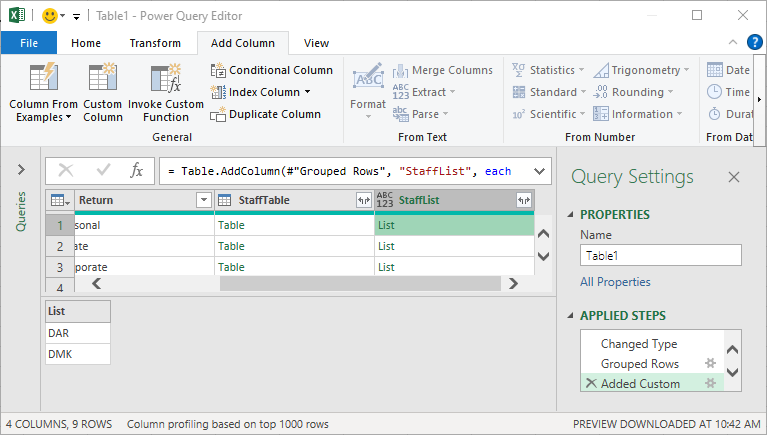
Think of each List as a little mini-list that contains a single column of staff assigned to each specific Client Return. We can see a preview of each list by clicking the empty space on any list cell:

We can now move to our next step.

Extract List – Separate Text Values

We want to convert each List into a single text value that we can send back to Excel. We have many options for combining the text values, including separating them with commas, colons, or spaces. In our case, we’ll use a comma-space to separate each.

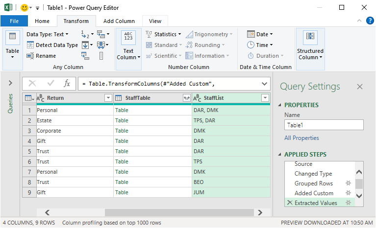
We select the entire StaffList column, and then click Transform > Extract Values. In the resulting dialog, we can pick any delimiter from the list, or define our own by selecting Custom. I’ve entered a comma followed by a space:

We hit OK, and bam:

Now, we remove the StaffTable column by selecting it and clicking Transform > Remove Columns. And with that, we can head to our next step.

Pivot Column

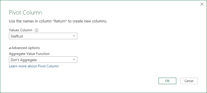
We select the entire Return column, and select Transform > Pivot Column. In the resulting Pivot Column dialog, we select StaffList as the Values Column. We then expand the Advanced options and select Don’t Aggregate (or Minimum or Maximum):

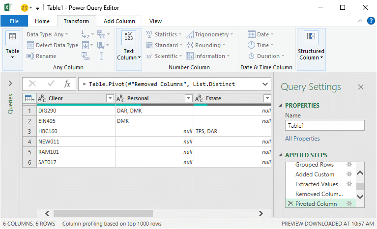
We hit OK, and bam:

Finally, we can send the results to Excel.

Return Data to Excel

We click Home > Close and Load To… and send the results back to a Table in the desired Excel worksheet:

Yay … we did it!

And the best part is that if the source data has any changes or new rows going forward, we don’t need to go through all of those steps again. We just need to right-click the results table and select Refresh!

Conclusion

I hope this alternative to a PivotTable report is useful when trying to display text values. If your workbook requires the use of a PivotTable, you can join text values together by using the data model and the CONCATENATEX DAX function. More info about that approach can be found here.

If this post was helpful, or if you have any suggestions for improvement or other alternatives, please share by posting a comment below!

Sample file