Excel Calendar with One Formula

In this post, we’ll see how to create an Excel calendar with a single formula. Specifically, we will write a formula that displays the days of any month in a graphical calendar format. Our graphical calendar displays the days of the specified month in 7 columns (Sunday through Saturday) and includes a row for each week. The key function in our formula is SEQUENCE, and it is the primary reason for the post. The other functions used in the formula help to ensure the days line up in the correct day column.

Objective – Excel Calendar

Before we get too far, let’s take a look at our desired outcome. We would like the user to be able to enter any month and year, like this:

And we’d like the calendar displayed in our worksheet like this:

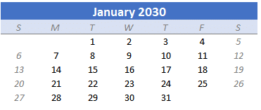
When a user enters a different month or year, we want Excel to automatically update the calendar.

Video Walkthrough

Narrative – Calendar Formula

We will create our calendar using the following three steps:

• Set up
• Formula
• Cosmetics

Let’s get to it.

Note: not all versions of Excel include the SEQUENCE function. The fastest way to determine if a version of Excel supports the SEQUENCE function is by typing =SEQ in any cell and seeing if SEQUENCE appears in the drop list. If your version of Excel does not support the SEQUENCE function, there are other approaches for creating a calendar discussed here and here.

Set up

Input Cells

First, we need to set up the input cells. We have two ways of doing this. We can allow the user to enter a month number and a year number into different cells, or have them enter a date into a single cell. Either way is fine.

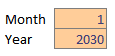
If you want to have them enter the month and year separately, create some labels like Month and Year and provide a couple of input cells next to them. If desired, apply the Input cell style (Home > Cell Styles > Input) to identify them.

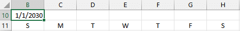
Another option is to allow the user to enter a date, like this:

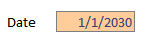
The key thing to note is that for the formula presented below to work properly, the date entered must be day 1 of the month, like 1/1/2030. If the user enters a day of other than the first day of the month, the formula below will produce unexpected results. You could address this issue by modifying the formula, applying data validation, or using other methods. But, in this post, we’ll just keep it simple and allow the user to enter the month and year separately.

Labels

Next, we’ll need to set up the basic calendar headers to display the month and year along with the days of the week. Eventually after we apply all of our cosmetics, we’d like them to look something like this:

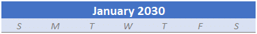
At this point in the process, we aren’t worried about their style and formatting, so they will look this this for now:

You’ll use a formula in B10 to display the date. If you opted to give the user a single date input cell (say in cell C5), you would use a direct cell reference like this:

=C5

If you opted to give the user separate year and month input cells (say in cells C6 and C5), you would use the DATE function like this:

=DATE(C6,C5,1)

We use 1 for the day argument so that it returns the first day of the month.

For the day labels, I just entered S, M, T, W, T, F, and S manually. You could just as easily enter three letter abbreviations such as Sun or other labels as desired.

With our set up complete, it is time to create our Excel calendar with a formula.

Excel Calendar Formula

Since this is Excel, there are many ways to write this calendar formula, and the solution presented is but one possible option.

SEQUENCE

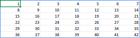
At the heart of this formula lies the SEQUENCE function. The SEQUENCE function returns a sequence of numbers. Let’s begin by looking at the first two arguments. They tell the SEQUENCE function how many rows and columns to create. For example, the following formula will create a range of 6 rows and 7 columns:

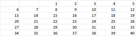
=SEQUENCE(6,7)

We hit enter and it creates this output:

In reality, this is pretty close to what we ultimately want. But, how do we ensure that the day numbers are displayed in the correct weekday columns? Well, if we are able to get the first day of the month to appear in the correct column, the remaining days will naturally fall in line. So, let’s get the first day of the month to appear in the correct weekday column.

WEEKDAY

For starters, we need to be able to determine the day of the week for the first day of the month. Fortunately, Excel has the WEEKDAY function which does just that. We provide it a date, and it tells us its weekday value. Since the cell we use to display our calendar header B10 already contains the date with the first day of the month, we can use this:

=WEEKDAY(B10)

By default, it returns 1 when the weekday is Sunday; 2 for Monday; and so on. There is an optional second argument you can use if you want to change the value returned based on the day, but in our case, the default is perfect.

Now that we know how to determine the weekday for the first day of the month, we need to use this information to update the original SEQUENCE function.

CHOOSE

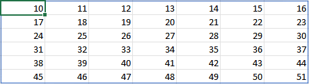
The third argument of the SEQUENCE function allows us to specify the starting number. For example, if we wanted the sequence to begin at the number 10 instead of the default 1, we could use this:

=SEQUENCE(6,7,10)

This would create this range:

In our case, we want the sequence to start at whatever number is needed in order to ensure that day 1 appears in the correct column.

For example, if the first day of the month is Sunday, we want our sequence to start at 1 so that the number 1 appears in the first cell (the Sunday column). However, if the first day of the month falls on a Monday, we want the sequence to begin at 0 so that 1 ends up in the second cell (the Monday column). If the first day of the month falls on a Tuesday, we want the sequence to begin at -1 so that 1 ends up in the third cell (the Tuesday column). And so on. There are multiple ways to approach this. The option we’ll discuss uses the CHOOSE function.

The following formula will return the results we need. Namely, it will return 1 when the weekday is Sunday; 0 when the weekday is Monday; -1 when the weekday is Tuesday; -2 when it is a Wednesday; and so on:

=CHOOSE(WEEKDAY(B10),1,0,-1,-2,-3,-4,-5)

Now, since this computes the correct sequence starting value, we can use it as the third argument of the SEQUENCE function, like this:

=SEQUENCE(6,7,CHOOSE(WEEKDAY(B10),1,0,-1,-2,-3,-4,-5))

We hit Enter, and bam … our Excel calendar formula is looking good:

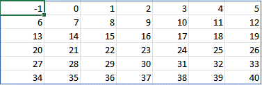
This is perfect because day 1 appears in the correct column.

With our days in the correct columns, all that remains is a bit of cosmetics.

Cosmetics

We’ll hide the day numbers that are not in the current month and style the calendar headers.

Hide day numbers

To hide the day numbers that aren’t in the current month, we’ll apply conditional formatting. We will create two separate rules … one to hide the numbers less than 1 and another to hide the numbers greater than the last day of the month.

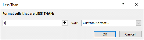
We select the entire calendar range and then Home > Conditional Formatting > Highlight Cell Rules > Less Than. In the resulting dialog, we enter 1 and the select Custom Format…

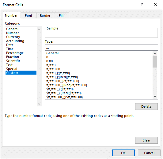
In the resulting Format Cells dialog, we select Custom and then enter three semicolons:

Bam:

Now, let’s hide the numbers that are greater than the last day of the month. Home > Conditional Formatting > Highlight Cell Rules > Greater Than. Then we enter the formula shown in the dialog below, which dynamically figures out the day number of the end of the month (last day of the month):

We use the same three semicolon custom format, and bam:

With our days appearing as desired, we can now revisit the calendar headers.

Headers

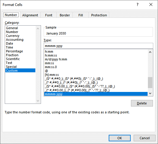
First, let’s adjust the date format of our calendar header cell B10. Instead of displaying a short date format, such as 1/1/2030, it should display the month name fully spelled out. We do this by selecting cell B10 and opening the Format Cells dialog. Then, we select Custom and enter mmmm yyyy like this:

We can then select all of the cells in the header row and open the Format Cells dialog again. Click Alignment > Center Across Selection > OK. Finally, we can apply any additional formatting desired, such as applying a cell style, bold font, or bigger font size.

If desired, we can apply the Explanatory Cell Style to the day labels and fill the cells as desired. We can also apply the Explanatory Cell Style to the Sunday and Saturday columns if desired. The resulting calendar looks like this:

Yay … we did it!

Now, the user can change the desired month and year for the calendar as desired. February 2030 would look like this:

March 2030:

And well … you get the idea 🙂

Conclusion

If you have any suggestions for how to improve this Excel calendar formula, or have any alternative formulas, please share by posting a comment below … thanks

Sample file

Additional Notes

Rather than using conditional formatting to hide the days that fall outside of the current month, we could wrap a TEXT function around our formula, like this:

=TEXT(SEQUENCE(6,7,CHOOSE(WEEKDAY(B10),1,0,-1,-2,-3,-4,-5))," [>"&DAY(EOMONTH(B10,0))&"];;#")

A slightly more compact version of the formula uses MOD instead of CHOOSE, like this:

=TEXT(SEQUENCE(6,7,-MOD(WEEKDAY(B10,2),7)+1)," [>"&DAY(EOMONTH(B10,0))&"];;#")