Mastering Excel’s PIVOTBY Function: A Dynamic Pivot Table Alternative

Sometimes, we need the flexibility of a PivotTable without actually building one. Whether we’re automating dashboards, preparing recurring reports, or just streamlining our workbooks, Excel’s PIVOTBY function gives us a powerful, formula-based solution. In this post, we’ll explore how to transform raw data into dynamic summary reports using a single formula — no PivotTable required.

Video

Tutorial

We’ll walk through how to:

• Create a summary report using a single PIVOTBY formula
• Use multiple value fields and aggregate functions
• Add subtotals and grand totals
• Apply dynamic formatting with conditional formatting
• Include category headers that auto-update with our data

Ready? Let’s dive in.

PIVOTBY

Before we jump in, let’s start with a summary of this function. PIVOTBY returns a dynamic array “summary table” that groups your data by the row/column fields you specify and aggregates the values using the aggregation function. The resulting report is similar to a PivotTable output, but created by a formula.

=PIVOTBY(row_fields, col_fields, values, function, [field_headers], [row_total_depth], [row_sort_order], [col_total_depth], [col_sort_order], [filter_array], [relative_to])

• row_fields: Column-oriented range or array used to group rows and generate row headers. Can include multiple columns for multiple row group levels.
• col_fields: Column-oriented range or array used to group columns and generate column headers. Can include multiple columns for multiple column group levels.
• values: Column-oriented range or array containing the data to aggregate. Can include multiple columns for multiple value fields.
• function: Aggregation function (e.g., SUM, AVERAGE, COUNT) or a lambda. Can be a vector of functions (for example, using HSTACK) to return multiple aggregations.
• field_headers (optional): Controls whether field headers are returned and displayed. Options include automatic detection, show, hide, or include headers in output.
• row_total_depth (optional): Controls row totals and subtotals.
• row_sort_order (optional): Controls row sorting. Positive numbers sort ascending, negative numbers sort descending. Can reference row fields or value columns.
• col_total_depth (optional): Controls column totals and subtotals (same logic as row_total_depth).
• col_sort_order (optional): Controls column sorting. Positive = ascending, negative = descending.
• filter_array (optional): A Boolean include/exclude array used to filter the source data before aggregation.
• relative_to (optional): Used with two-argument aggregation functions (such as percent calculations) to define what totals the calculation is relative to (e.g., row total, column total, grand total).

Creating a Basic Pivot-Style Report with PIVOTBY

We’ll start simple. Suppose we have a table named Table1 with columns: Region, Quarter, and Revenue like this:

Our goal is to summarize revenue by region with quarters across the top (in columns).

We can use the following formula:

=PIVOTBY(Table1[Region], Table1[Quarter], Table1[Revenue], SUM)

This function uses the following arguments:

• Row field: Region
• Column field: Quarter
• Value field: Revenue
• Aggregate function: SUM

Just like that, we get a pivot-style summary of revenues across quarters by region — with one formula:

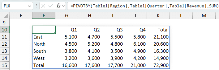
Because this is a dynamic array function, it updates automatically when the source data changes or when new rows are added.

Using Multiple Value Fields

What if we have more than one metric to summarize? Say we have Department, Salary, and Bonus:

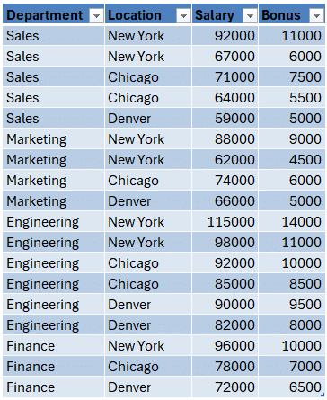
Here’s how we can return both in the same report:

=PIVOTBY(Table2[Department],, Table2[[Salary]:[Bonus]], SUM)

This shows the total salary and bonus by department:

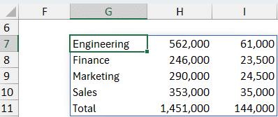
Notice we didn’t include column fields, which is perfectly valid. PIVOTBY allows flexibility in how we group and analyze our data.

Using Multiple Aggregate Functions

It’s also possible to apply different aggregation methods to the same measure. For example, we can show both the sum and percent of total salary by department:

=PIVOTBY(Table2[Department],, Table2[Salary], HSTACK(SUM,PERCENTOF))

Bam:

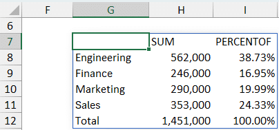
Using HSTACK within the aggregate function argument allows for side-by-side metrics.

Summarizing with Multiple Row Fields and Subtotals

Let’s take it up a notch.

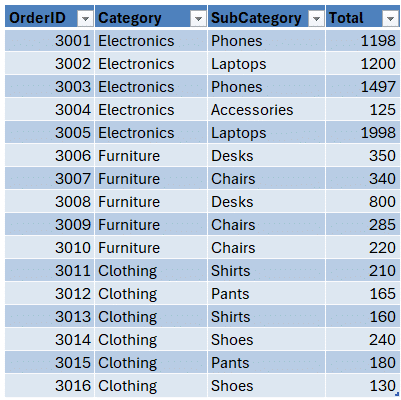
Suppose we’re analyzing Category and Subcategory, with a Total column. Here’s how we do that:

=PIVOTBY(Table4[[Category]:[SubCategory]],,Table4[Total],SUM)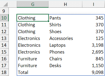

The optional 6th argument — RowTotalDepth — controls whether subtotals and grand totals are included:

• 0: No totals
• 1: Grand totals only
• 2: Both subtotals and grand totals

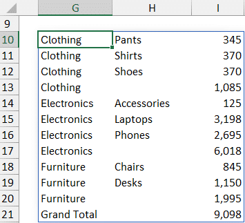
So, if we wanted to show subtotal, we could update our formula like this:

=PIVOTBY(Table4[[Category]:[SubCategory]],,Table4[Total],SUM,,2)

And bam:

Dynamic Conditional Formatting for Totals

Since our output range changes based on the formula, static formatting won’t work reliably. Instead, we’ll apply conditional formatting. Here’s how:

To bold grand totals:

1. Select the output columns (e.g., G:I)
2. Note: when you select columns G:I, one cell (probably G1) will be “active”; if a different cell is the active cell, update step 4 below to reference the active cell with an absolute column reference ($G) and a relative row reference (1)
3. Go to Conditional Formatting > New Rule > “Use a formula to determine…”
4. Enter:
   =$G1="Grand Total"
5. Apply bold formatting and a bottom cell border

To bold subtotals:

1. Repeat the steps above
2. Formula:
   =AND($G1<>"", $H1=""))
3. Apply your desired format (bold + bottom cell border)

Apply these formulas and bam:

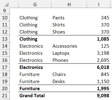
These subtle visual cues help readers distinguish between detail rows, subtotals, and grand totals — and because it’s conditional formatting, the style stays consistent no matter how rows shift.

Wrapping It Up

The PIVOTBY function is a powerful alternative to traditional PivotTables, especially when we want the results in a single-cell formula. It simplifies automation, simplifies formatting, and adapts to data changes instantly. When paired with HSTACK and conditional formatting, we can generate beautifully structured, always-up-to-date reports.

If this deep dive into PIVOTBY has helped simplify your reporting process, keep exploring! This function has many arguments that can help you customize your report far beyond what we’ve discussed in this short post.

Sample Workbook

FAQs

1. Q: What version of Excel supports PIVOTBY?
   A: PIVOTBY is currently available in Excel 365.
2. Q: Can I combine multiple row and column fields?
   A: Absolutely. Just select them directly (if adjacent and in the desired order) or use CHOOSECOLS.
3. Q: How do I use multiple aggregation functions?
   A: Wrap the aggregation function names in HSTACK; for example, HSTACK(SUM,PERCENTOF).
4. Q: Can PIVOTBY be used with filters?
   A: Yes, filters can be added as one of the optional arguments — great for focusing on subsets of your data.
5. Q: Can I format PIVOTBY output dynamically?
   A: For dynamic reports, use conditional formatting rather than static number formatting.
6. Q: Is PIVOTBY better than PivotTables?
   A: This function is not more powerful that PivotTables. But, they are a nice alternative for basic reports.
7. Q: Can I sort results generated from PIVOTBY?
   A: Sorting can be controlled using optional sort order parameters in the function.
8. Q: Is the result array spill-safe?
   A: Yes, but ensure there’s space below and to the right of the formula cell to allow the dynamic array to expand.
9. Q: How do I update results if data changes?
   A: You don’t have to! As a dynamic array function, PIVOTBY auto-updates whenever the source data changes.