Build Advanced Excel Formulas Instantly with the Claude Add-In

What if we could describe what we want in plain English and Excel builds the formulas for us?

In this post, we’ll explore how to use the Claude Excel add-in to generate dynamic formulas, lookup models, and summary reports in seconds.

Video

Tutorial

We’ll walk step-by-step through three practical exercises that demonstrate how AI can accelerate formula development while still allowing us to verify and control the results.

Our goal isn’t to replace Excel skills … it’s to accelerate initial time to draft.

Let’s dive in.

Step 1: Install the Claude Excel Add-In

Before we begin building formulas, we need to install the add-in.

1. Go to Home → Add-ins.
2. Search for Claude.
3. Click Add and log into your account.

You will then login to your account.

Note: as of now, a paid Claude subscription is required. More info at claude.com. Claude is a service by a company called Anthropic, and is not affiliated with Microsoft.

Once you have installed the add-in and logged in with your account, it appears in the side panel, like this:

We can prompt Claude to:

• Build financial models
• Explain a workbook
• Transform messy data
• Debug formulas
• Or execute custom prompts

Now let’s put it to work.

Exercise 1: Dynamic Customer Dashboard with XLOOKUP and SUMIFS

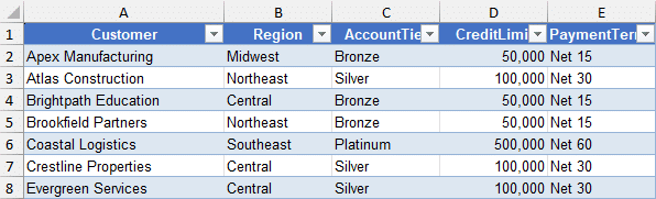
Data

We have a data table (Sales) that looks a bit like this:

We also have a customer lookup table (Cust) that looks like this:

Objective

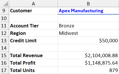
In a new worksheet, we want to:

• Create a customer dropdown
• Return Account Tier, Region, and Credit Limit from a lookup table
• Calculate total Revenue, Profit, and Units for the selected customer
• Use dynamic formulas only

Important: Region does not exist in the transaction table. That means we must use a lookup based on Customer.

Prompting Claude

We provide a prompt summarizing what we want. Something like this:

Create a dropdown so I can pick a customer. Write a formula that looks up the selected customer from the Lookups table and returns their Account Tier, Region, and Credit Limit. Also give me the total revenue, profit, and number of units for that customer. This should all be done with dynamic formulas, so I can pick any customer and the formulas will update.

We hit enter, and Claude gets to work. It evaluates the entire workbook, data, formulas, creates a plan, and generates:

• Data validation dropdown
• XLOOKUP formulas for Account Tier, Region, Credit Limit
• SUMIFS formulas for totals

The formulas it writes to retrieve the Account Tier, Region, and Credit Limit from the lookup table use XLOOKUP, a bit like this:

=XLOOKUP(B9,Lookups!A:A,Lookups!C:C,"Not Found")

The formulas it writes to aggregate the Total Revenue, Profit, and Units look a bit like this:

=SUMIFS(Data!I:I,Data!C:C,B9)

Pretty good, but a bit different than I would have done in practice. I would have definitely used the same functions, XLOOKUP and SUMIFS for these tasks, but I would have used the structured table references (Table1[Revenue]) instead of the whole-column references (Data!I:I) in the function arguments. Both options return the same results at this time, but my preference is to use the Table name in case we enter some values above or below the data range down the road that we do not want included in the results.

Spot-Checking the Results

Now, let’s verify the AI results (always!)

We spot check the related value retrieved with XLOOKUP from the lookup table, all good.

Then, we check the aggregated values by filtering the data by the selected customer and compare the total row for:

• Total Revenue
• Total Profit
• Total Units

Good news: the AI formulas returned the correct values.

Recap

Key takeaway: the AI formulas returned accurate values. I would have used different references inside my formulas (Structured Table References instead of whole column references), I would have chosen different columns (B:C instead of A:B), and I would have chosen different formatting (no currency symbol $). These are of course personal preferences which are relatively quick to update.

Exercise 2: Region Summary Report (Formulas Only, No PivotTables)

Objective

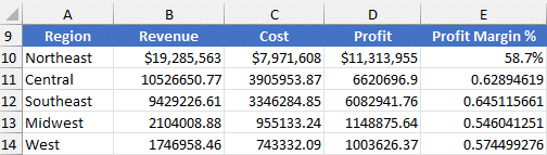
We want a summary report showing:

• Total Revenue by Region
• Total Cost
• Total Profit
• Profit Margin
• Sorted from highest to lowest Revenue
• No PivotTables allowed

Note: to determine this by region, a relationship between the lookup and data table is needed. This is because Region is not located directly in the data table. It is only through the customer column that you can determine region.

Prompt

Build a summary report that shows total Revenue, Cost, and Profit by Region, sorted from highest to lowest Revenue. Include a column for Profit Margin %. Use formulas only (no pivot tables). Build with formulas so if I change the data the report will update.

What Claude Built

All regions spill automatically, sorted descending by Revenue.

Claude created a dynamic spill formula using modern Excel functions:

• LET
• XLOOKUP
• UNIQUE
• BYROW
• LAMBDA
• SUMPRODUCT
• SORTBY

Claude didn’t format these columns, but that is very quick to update. Here is the formula it used for the Region column:

=LET(regions,XLOOKUP(Data!C2:C3201,Lookups!A:A,Lookups!B:B),
uRegions,UNIQUE(regions),
rev,BYROW(uRegions,LAMBDA(r,SUMPRODUCT((regions=r)*Data!I2:I3201))),
SORTBY(uRegions,rev,-1))

It used similar formulas for the remaining columns. These would have taken me longer than Claude to figure out, I’m sure.

Verification

We perform a sanity check:

• I noted the grand total in the data
• I compared it to the report total

All totals match perfectly!

Everything updates dynamically as data changes.

This is a powerful example of building a PivotTable-style report using formulas only.

Recap

If this were my project, I would be tempted to add a Region helper column to the data table, and then use the GROUPBY function, like this:

=GROUPBY(Sales[Region],Sales[[Revenue]:[Profit]],SUM,0,1,-2)

If I weren’t allowed to add a helper column, I would have nested GROUPBY/XLOOKUP into this single formula:

=GROUPBY(XLOOKUP(Sales[Customer],Cust[Customer],Cust[Region]),
Sales[[Revenue]:[Profit]],SUM,0,1,-2)

Although, technically this doesn’t include the profit margin.

So, again, I would have personally opted for a different approach, however, Claude’s numbers were indeed accurate.

And I think this is just a fact about Excel … there are many ways to accomplish any given task. Some Excel users prefer VLOOKUP, others XLOOKUP, while others INDEX/MATCH. So, it doesn’t surprise me that AI opts for a different approach than I would here.

Exercise 3: Top and Bottom Transactions by Category

Objective

We now want:

• A Category dropdown
• Top 3 transactions by Revenue
• Bottom 5 transactions by Profit
• Fully dynamic output

Prompt

Create a dropdown for Category. Then give me the top 3 transactions in the selected category by revenue. Also show the bottom 5 transactions based on profit.

How Claude Solved It

Claude’s results:

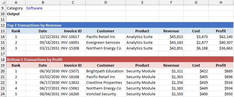
Each section is powered by a single spill formula.

Claude used a combination of:

• LET
• FILTER
• CHOOSE
• SORT
• TAKE

Here is an example of the formula it used in B14:

=LET(cat,$B$9,
filt,FILTER(CHOOSE({1,2,3,4,5,6,7},Data!A$2:A$3202,Data!B$2:B$3202,Data!C$2:C$3202,Data!D$2:D$3202,Data!I$2:I$3202,Data!J$2:J$3202,Data!K$2:K$3202),Data!E$2:E$3202=cat),
sorted,SORT(filt,5,-1),
TAKE(sorted,3))

Spot-Checking Again

I compared the values to the data, and once again, they were 100% accurate.

I also changed the drop-down, and sure enough the report updated accordingly.

This confirms:

• The logic is correct
• The sorting works
• The formulas are dynamically linked

Recap

If this were my project, I would have probably used this formula instead:

=TAKE(SORT(CHOOSECOLS(FILTER(Sales,Sales[Category]=B9),1,2,3,4,9,10,11),5,-1),3)

This time, I really did like the formatting Claude applied!

What We Learned About AI in Excel

Here’s the big picture:

• AI builds complex formulas quickly
• It uses modern Excel functions
• It may use a different approach than I would
• It may need small corrections, especially in structure and formatting
• Spot-checking remains essential! (Never blindly trust an AI lol)

The numbers were consistently accurate. The structure sometimes needed refinement, but that’s a small tradeoff for the time saved.

Think of Claude as a formula assistant, not a replacement for Excel expertise.

Final Thoughts

The Claude Excel add-in demonstrates how AI can dramatically simplify advanced Excel formula creation. By combining natural language prompts with modern dynamic array functions, we can build dashboards, reports, and ranking systems faster than ever.

AI gives us speed. Excel knowledge gives us confidence. And verifying results remains critical.

File Download

Download the completed workbook used in this tutorial:

Frequently Asked Questions

1. What is the Claude Excel add-in?

It’s an AI-powered add-in that allows us to generate formulas, models, and reports using natural language prompts.

2. Does Claude replace the need to know Excel formulas?

No. It accelerates development, but we still need to understand and verify results.

3. What functions did Claude use in these examples?

XLOOKUP, SUMIFS, SUMPRODUCT, SORT, FILTER, CHOOSECOLS, and CHOOSEROWS.

4. Can we build reports without PivotTables using AI?

Yes. As shown, Claude created a fully dynamic region summary using formulas only.

5. Is the output dynamic?

Yes. Results update automatically when selections change.

6. Should we trust AI-generated formulas without checking?

No. Always spot-check totals and logic against the source data.

7. Can Claude fix formula errors?

Yes. We can prompt it to debug or correct issues like broken data validation.

8. Is this better than writing formulas manually?

It’s faster to get a preliminary result; but understanding the formulas and verifying the results remains critical.

9. What’s the biggest benefit of using AI in Excel?

Speed. We can generate a working first draft in seconds and refine from there.