GROUPBY

Microsoft Excel continues to evolve, and one of the most impressive additions to the Excel formula family is the GROUPBY function. With it, we now have the power to create fully dynamic and flexible summary reports—all with a single formula. If you’ve relied on pivot tables or manual formulas for reporting, you’re going to love this streamlined approach. Let’s walk through how to use GROUPBY in Excel to simplify your summary reports.

Video

What Does GROUPBY Do?

The =GROUPBY() function allows us to aggregate data—like totals or averages—based on one or more fields. Think of it like a PivotTable, but embedded into a formula that updates dynamically. Whether you’re working with raw ranges or structured tables, GROUPBY supports grouping, filtering, and sorting, all inside of one concise formula.

Creating a Basic Summary Report with GROUPBY

Let’s say we have a dataset that includes products and their sales figures.

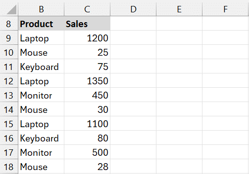
Our goal is to create a simple summary report showing the total sales per product.

Enter the following formula into E8:

=GROUPBY(B9:B18, C9:C18, SUM)

Arguments Explained:

• Row Fields: The field(s) we want grouped (e.g., Product)
• Values: The numeric field we want aggregated (e.g., Sales)
• Function: The aggregation logic (e.g., “SUM”, “AVERAGE”, “MAX”, etc.)

And bam:

A summary report with a single formula!!

Adding Header Options

The fourth argument allows us to handle headers in our range:

• 0: No headers
• 1: Headers included, but not shown
• 2: Headers not present, but generated
• 3: Headers included and shown

=GROUPBY(A1:A10, B1:B10, SUM, 3)

This tells Excel that our data includes headers and we want them shown in the result:

Controlling Totals with Total Depth

Argument 5 controls total rows such as grand totals or sub-totals:

• 0 – No totals
• 1 – Grand totals only
• 2 – Subtotals (only works with multiple row fields)
• 3 – Grand totals at the top

=GROUPBY(A1:A10, B1:B10, SUM, 3, 1)

Sorting the Results

Argument 6 lets us define sorting:

• 1 sorts ascending by the first column
• -1 sorts descending by the first column
• 2 sorts ascending by the second column
• -2 sorts descending by the second column

=GROUPBY(A1:A10, B1:B10, SUM, 3, 1,-2)

This gives us the flexibility to order the output by the metric or the grouped value.

Multiple Grouping Fields

Let’s say our data includes multiple columns, and is stored in a table named Table1, like this:

Need to group by Region and then by Product? Simply select both columns in the first argument.

=GROUPBY(Table1[[Region]:[Product]],Table1[Sales],SUM)

Bam:

This provides a summary by region and then within each region by product.

Add Dynamic Filtering With Filter Array

Want to filter the data before aggregating?

The 7th argument lets us supply a Boolean array to include/exclude rows.

=GROUPBY(Table1[[Region]:[Product]],Table1[Sales],SUM,,,,Table1[Region]="East")

This formula will summarize only the data where the region is East:

Change Grouping Order with CHOOSECOLS

Want to flip the order of your grouping? Use CHOOSECOLS to re-order the fields dynamically:

=GROUPBY(CHOOSECOLS(Table1,2,1),Table1[Sales],SUM)

This reverses the grouping from Region > Product to Product > Region:

Controlling Hierarchical Display

The 8th argument changes how group hierarchy is handled:

• 0 – Hierarchy (default)
• 1 – Table

If we sort by column 2, no apparent changes to sort order (it still sorts by column1 region):

=GROUPBY(Table1[[Region]:[Product]],Table1[Sales],SUM,,,2)

This is because the default value for the field_relationship argument (8th argument) is 0 which means Heirarchy. Let’s change it to 1 for Table:

=GROUPBY(Table1[[Region]:[Product]],Table1[Sales],SUM,,,2,,1)

Now we can see it sorts by column 2 product!

Formatting the Summary Dynamically

Static formatting doesn’t play well with dynamic formulas. Instead, we can use Conditional Formatting to format totals based on logic:

Select the columns that contain the summary report (here, columns F:H). Then:

1. Home > Conditional Formatting > New Rule
2. Select “Use a formula to determine which cells to format”
3. Enter the formula: =($F1="Total")
4. Apply desired format (e.g., top border)

This adds formatting only to the Total rows and automatically updates as your formula output adjusts. You can also format column H to include the thousands separator, and add the headers … bam:

Now we have a fully dynamic summary report … yay!

Summary

The GROUPBY function is a powerful addition to Excel’s toolkit. It simplifies data summarization, eliminates the need for PivotTables in some cases, and can handle grouped, filtered, and sorted views with a single formula. When combined with CHOOSECOLS and conditional formatting, we can build highly customized and dynamic summary reports that update automatically as source data changes.

If you’re excited about integrating GROUPBY into your Excel workflow, be sure to download the example file and explore how it can change the way you build reports!

Download the Example File

We’ve created a downloadable Excel file packed with each exercise and formula shown in this post.

Frequently Asked Questions

1. What versions of Excel support GROUPBY?

GROUPBY is available in Excel 365 and Excel 2021 (for Microsoft 365 users only).

2. Can GROUPBY replace PivotTables?

In some cases, yes! GROUPBY lets you build dynamic summary reports entirely with formulas. If you need column values, check out the PIVOTBY function instead.

3. Can I group by multiple columns?

Absolutely. Just select multiple columns as the first argument or use CHOOSECOLS to arrange them dynamically.

4. Can I use GROUPBY with named Tables?

Yes, GROUPBY works seamlessly with Excel Tables, making references easier and cleaner.

5. How do I sort by total instead of grouped fields?

Use the 6th argument to specify sort column as the values column.

6. How to filter data within GROUPBY?

Use the 7th argument with a Boolean array such as Region="East" to limit data inclusions.

7. What aggregate functions can I use?

GROUPBY supports SUM, AVERAGE, MAX, MIN, COUNT, and more out of the box.

8. Can I customize the column headers?

Yes, use the 4th argument to show/hide/generate headers as needed.

9. How dynamic is the final output?

Fully dynamic! The output updates automatically when source data changes—no refreshing needed.

10. Is GROUPBY volatile?

No, it’s not considered volatile and won’t recalculate unnecessarily.