Excel University Blog
Read on for in-depth articles, tutorials, and videos. Search or browse for specific topics. Be sure to subscribe if you'd like to be notified when we write something new.
Features

Excel has cell formatting designed just for accountants. Not surprisingly, it is called the Accounting Number Format. The built-in ribbon commands apply the format with two decimals and the currency symbol. This post demonstrates how to set up two handy QAT icons so that we can quickly apply this format with no decimals and without a currency…
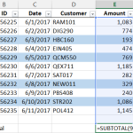
If you need to compute the total for certain cells based on their font or fill color, you may have noticed that Excel formulas operate on stored values, not displayed values. That means that functions such as SUM and SUMIFS operate on the underlying cell values and disregard cell formatting, such as font or fill…
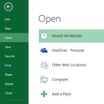
I’m not sure about you, but, sometimes I sort of miss the old days of Excel when Ctrl+O immediately displayed the Open dialog box. This dialog box allowed me to quickly navigate my computer and find the file I wanted to open. However, when Microsoft introduced the Backstage, this keyboard shortcut stopped displaying the Open…

Are you familiar with the double-click shortcut to fill formulas down? If so, have you noticed it stops filling down at the first blank row? This post will discuss the double-click shortcut as well as a simple workaround for how to fill it down through a report range even when there are blank rows in…

When you need to compute a future date and exclude weekends, you may want to consider exploring the WORKDAY function. In this post, we’ll use the WORKDAY function to prepare a simple project plan and then display it with a Gantt chart. Objective We have a project that we are managing and it has several…
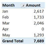
If you have ever created a PivotTable report that groups by month, you may have encountered an awkward situation where the PivotTable only displays the months that actually have data in the source. The PivotTable will summarize the data that exists and if there are no transactions for a given month, the PivotTable won’t display it.…

If you haven’t checked out Excel’s conditional formatting feature recently, you’re missing out on some nice enhancements. The feature formats a cell based on its value. Excel continuously monitors the cell value and updates the formatting as the cell value changes. Conditional formatting has traditionally been limited to basic cell formatting such as fill and…

With a simple custom format code, we can display negative numbers as positive…but…why would we want to? So that we can simplify our formulas and make our workbooks more reliable of course. Let’s check it out. Objective Before we get to the mechanics, let’s confirm our goal. We have a worksheet, in this case a little…

In this post, we’ll perform a two-dimensional lookup with Excel’s VLOOKUP function. Objective Let’s begin by clarifying our objective and what is meant by the term two-dimensional lookup. We have stored our price list in a table, and the price for each item varies based on the region. This is illustrated in the screenshot below. To…

Did you know that PivotTables can automatically group date fields by month? And by quarter and year? This date group capability makes it easy to summarize data in monthly columns without writing a single formula. Check out my recent California CPA Magazine article for the details. Publication: California CPA Magazine Author: Jeff Lenning CPA Date: May 2015…