Show PivotTable Months without Data
If you have ever created a PivotTable report that groups by month, you may have encountered an awkward situation where the PivotTable only displays the months that actually have data in the source. The PivotTable will summarize the data that exists and if there are no transactions for a given month, the PivotTable won’t display it. A common workaround is to add empty data rows for each desired month into the data source to force the PivotTable to display all desired periods. However, this workaround isn’t necessary, and in this post, we’ll discuss a simple setting that will cause Excel to display all months, including those that have no underlying data transactions.
Objective
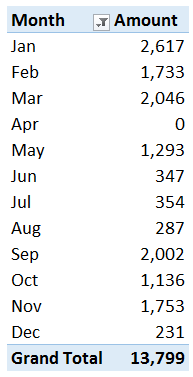
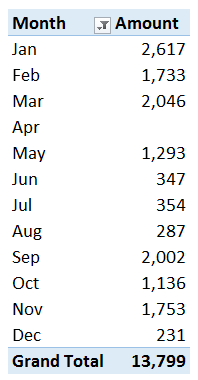
Our objective is rather simple, we want to create a PivotTable that displays the total amount by month for all months, including any months without data. This is illustrated in the screenshot below where April has no transactions in the data source.
Let’s build this thing.
Steps
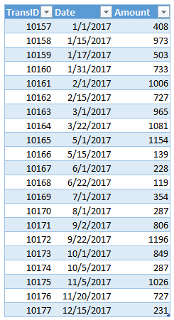
The underlying data table that we want to summarize is shown below.
Note: there are no data rows for April.
Here are the steps to build the desired PivotTable report:
- Create basic PivotTable
- Group by month
- Check the Show items with no data checkbox
- Filter the report
- For empty cells show 0
Let’s dig into the details of each step.
Create the basic PivotTable
To build the basic PivotTable, we select any cell in the data table, and then use the Insert > PivotTable ribbon icon. In the resulting Create PivotTable dialog box we tell Excel to place the report on the desired worksheet and click OK.
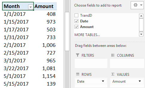
Then, we insert the Date field into the Rows area and the Amount field into the Values area. If desired, we can apply some cosmetic touches such as formatting the value field to include commas and updating the report headers. The resulting report is shown below.
Group by month
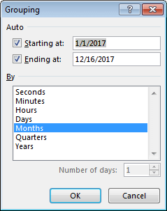
Now we need to tell Excel to group the report labels by month. We select any date cell in the report and then click the PivotTable Tools > Group Selection ribbon icon or we right-click a date cell and select Group. In the resulting Grouping dialog box, we accept the default selection of Months and click OK.
We are getting closer! The resulting report is shown below.
The big problem at this point is that there is no report label for April. This is because there are no April transactions in the PivotTable’s data source. This is where we use the Show items with no data checkbox.
Show items with no data checkbox
We open up the Field Settings dialog for the Date field either by selecting a month cell and then using the PivotTable > Field Settings ribbon icon or by right-clicking a month cell and then selecting Field Settings.
On the Layout & Print tab, we check the Show items with no data checkbox, as shown below.
Yes…the report now includes an April label as shown below.
The hard work is now complete and we just need to clean it up a bit.
Filter the report
Let’s filter out the report endpoints (<1/1/2017 and >12/16/2017) by using the filter drop-down and unchecking these items. Looking better. The updated version of the report is shown below.
For empty cells show 0
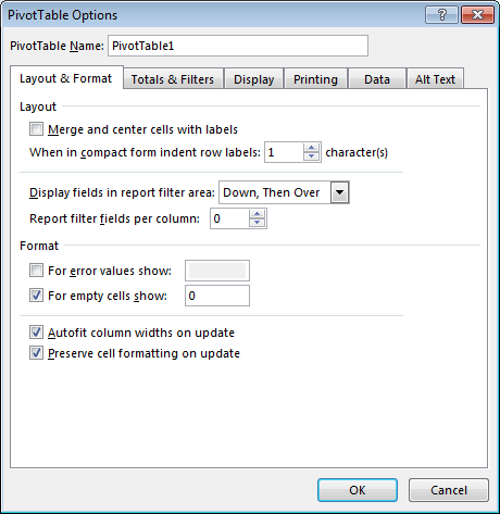
The final step is to show 0 for April. This is done in the PivotTable Options dialog box. We open it by clicking any cell in the report and then using the PivotTable Tools > Options ribbon icon or by right-clicking any cell in the report and selecting PivotTable Options.
In the PivotTable Options dialog, we type 0 into the For empty cells show field, as shown below.
We did it…yay! The resulting PivotTable is shown below.

This report shows 0 for April, even though there are no April transactions in the data source. We accomplished our objective!
If you have any other ideas about using the Show items with no data checkbox, please share by posting a comment below…thanks!
Additional Resources
- Sample Excel file
- Month Groups article
- Also works with intervals such as discussed in this histograms post
- Other Excel University posts about PivotTables
Excel is not what it used to be.
You need the Excel Proficiency Roadmap now. Includes 6 steps for a successful journey, 3 things to avoid, and weekly Excel tips.
Want to learn Excel?
Our training programs start at $29 and will help you learn Excel quickly.



Thank you!!!!!!
Welcome 🙂
Hello
Thanks! Very helpful article!
I am using Excel 2011 for Mac and cannot find the “Show items with no data” option in the individual fields but only at the PivotTable Options dialog and still, it appears as grayed (disabled) and not sure how to use it. There are two checkboxes for Display items with no data “on rows” and “on columns” but both are disabled.
Could you help?
Thank you!
Hi Isabel! I’m so sorry, but I don’t happen to have a copy of Excel 2011 for Mac so I’m unable to be of much help. Excel’s features and options are often based on the version, so, it could be that this option isn’t available in that version of Excel.
Best if luck,
Jeff
Thanks for the article. Very clear.
Do you know of any tricks to add a year to the month display above? My reports always nee the LAST 12 months, so I’d like the left column to be “Jul 15” instead of “Jul”
Hey Jim
I was unable to find EXACTLY what you need because Excel only formats a group in one way. I couldn’t change the format, and if I changed the format of the date in the data, the Pivot Table would not display each month only once. It also wouldn’t show only subtotals as to have each month only once.
The closest I could find was to group the date field by year as well as month, show the report in tabular form, and repeat all labels. I also turned off the +/- buttons and got:
2017 Jan ###
2017 Feb ###
2017 Mar ###
and so on…
Let me know if that isn’t what you are looking for and if I can be of further help:)
Kurt LeBlanc
Kurt:
Thanks for the response. Fighting storms at home right now so I apologize for being slow to acknowledge. The easiest work around I have found to date is to make an extra column in the source data with the format I want as a text field: =text(date,”mmm ‘yy”).
Jim
Hey Jim,
I understand:)
OK great! I’m glad you found a way that works for you.
Kurt LeBlanc
Does “show items with no data” work for dates as well as months? It doesn’t seem to for me. I have this data:
Date Session # Tables Session
Thursday, January 22, 2015 10 22.5 Thu Morn
Thursday, January 22, 2015 12 4.0 Thu Eve
Friday, January 23, 2015 13 34.0 Fri Morn
Saturday, January 24, 2015 17 24.5 Sat Aft
Sunday, January 25, 2015 21 13.0 Sun Eve
Monday, February 2, 2015 1 9.0 Mon morn\
Note that dates January 26-31 are missing.
When a create a pivot table to show tables by day, it does not include the missing days, even after I check that box. It doesn’t seem to update the table after I check that box.
Any help?
Yes…The “show items with no data” option works on grouped fields. Fortunately, you can group by Days. In the Grouping dialog, select Days and then define the start and end dates. Once the date field has been grouped, then the “show items with no data” option will take effect, and display an item for each date in the range.
Hope it helps!
Thanks,
Jeff
Thanks. It works!
Welcome 🙂
Thank you for this Article with clear instructions.
Thanks for this!!! I’ve been searching for this solution for some time!
THANKS!
Brilliant, inspirational, this has made my day and saved me a great deal of work. THANK YOU!!!
Welcome 🙂
I want to have a report with the months across the top horizontally and I want every month to show even though we’re only in January at this time. Your trick here worked when the dates were in rows, but I can’t get it to work when they are in columns. The Group feature is available but being able to specify the date ranges of 1/1/2-18 to 12/31/2018 is not available. Any ideas?
i love u for this !!!!
my hours of wasting in duplicating rows has come to an end !!!!
Thank You!!!
show ITEMS WITH NO DATA works with Rows only…can it be done with Columns???