Macro to Quickly Format PivotTable Values

PivotTable users frequently spend time assigning the same number format to PivotTable values. To my knowledge, there isn’t a built-in setting that allows us to define a default value field format. But, it is pretty easy to set up a macro that instantly assigns a desired format. This post walks through the steps of creating such a macro.

Objective

Generally, PivotTable value fields are automatically assigned the General format, as shown below.

To clean up the report, we manually change the format of the value field, to something such as a number, no decimals, with a comma, as shown below.

Rather than perform this task manually for each value field in each PivotTable we create, we can set up a macro to apply a specific format.

Detailed Steps

Overall, we’ll use the macro recorder to have Excel prepare a basic starter macro and save it in the Personal Macro Workbook. Then, we’ll modify the macro so it can be used on new PivotTables going forward.

Our steps will be:

• Record a macro that formats a cell
• Edit the macro
• Set up a QAT button
• Clean up

Let’s get started.

Record a macro

We will ask Excel to watch us apply the desired format to any random cell and save the recording in the Personal Macro Workbook. To do this, we simply start the macro recorder by clicking the following ribbon command:

• View > Macros > Record Macro

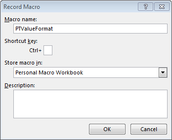
In the resulting Record Macro dialog box, we assign a name, avoiding spaces and funky characters, and opt to store the macro in the Personal Macro Workbook, as shown below.

Now…I mean right now…Excel is watching everything you do. So, simply apply the desired number format to the cell that is currently active. You can use any of the standard methods to apply your desired format.

Here, I opened the Format Cells dialog with Ctrl+1, and then assigned a number format, no decimals, with a comma.

Then, STOP the recorder. You can do this with the following ribbon command:

• View > Macros > Stop Recording

Step one is now complete. Since our macro simply formats the active cell, we need to make it a little bit smarter.

Edit the macro

We need to update the macro and tell it to apply this format to all PivotTables on the active worksheet. Since the macro is stored in the Personal Macro Workbook, we’ll need to first unhide this workbook in order to edit the macro.

To unhide the Personal Macro Workbook, simply click the following ribbon icon:

• View > Unhide

In the resulting Unhide dialog box, select PERSONAL.XLSB as shown below.

With the Personal Macro Workbook visible, we can now edit any macros it contains. To do so, we’ll open the Macro dialog by clicking the following ribbon icon.

• View > Macros > View Macros

In the resulting Macro dialog box, as shown below, we simply pick our new macro and click the Edit button.

Doing so opens the Visual Basic Editor and places the cursor inside our new macro, as shown below.

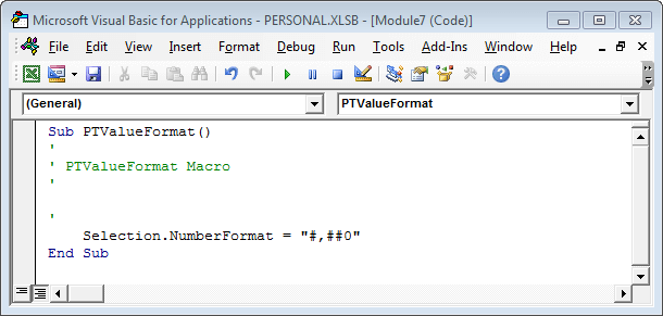
The macro simply applies the specified number format to the active cell. We want our macro to apply this formatting to all value fields in all of the PivotTables on the active worksheet.

Thus, we’ll make a few changes, as follows.

Sub PTValueFormat()
  For Each pt In ActiveSheet.PivotTables
    For Each df In pt.DataFields
      df.NumberFormat = "#,##0"
    Next df
  Next pt
End Sub

Note: you can copy the code above and paste it into your visual basic editor instead of typing it. 

Or, we could add an additional loop so that the macro assigns the format to all value fields, in all PivotTables, on all sheets in the active workbook. Here is the code for that version.

Sub PTValueFormatAllSheets()
  For Each ws In ActiveWorkbook.Worksheets
    For Each pt In ws.PivotTables
      For Each df In pt.DataFields
        df.NumberFormat = "#,##0"
      Next df
    Next pt
  Next ws
End Sub

Now, anytime we run this macro, Excel will apply the desired format to the PivotTable value fields. Let’s make the macro easy to run by setting up a QAT icon.

QAT button

To set up a QAT (Quick Access Toolbar) icon, we simply open the Excel Options dialog with the following:

• File > Options

Click the Quick Access Toolbar category on the left side of the dialog, and then you want to Choose commands from Macros, as shown below.

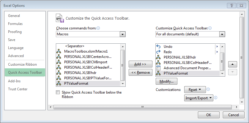
Select the new macro in the left list box and then click the Add button. The macro will appear in the right list box, and then you click OK to close the dialog.

Now, anytime you want to assign the desired format to your PivotTable value fields, just click the new QAT icon.

Clean up

Since we previously used the Unhide command to show the Personal Macro Workbook, we’ll probably want to hide it again. To do so, make it the active workbook and then click the following ribbon icon:

• View > Hide

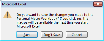
Also, since we want to save our new macro, we’ll want to be sure to click Save to the following dialog when existing Excel.

And that is how to set up a macro to apply a desired format to PivotTable value fields. If you have any other fun PivotTable formatting tricks or formatting macros, please share by posting a comment below…thanks!

Resources

• Sample file with macro: PTValueFormat