Excel University Blog
Read on for in-depth articles, tutorials, and videos. Search or browse for specific topics. Be sure to subscribe if you'd like to be notified when we write something new.
Excel

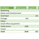
We are right in the middle of a blog series called VLOOKUP Hacks. We started by exploring the 4th VLOOKUP argument. Then we hacked the 3rd argument. Now, as you may have imagined, it is time to hack the 2rd argument. In this post, we’ll allow the user to retrieve values from different lookup tables.…
This is the 4th post in the VLOOKUP Hacks series. The first three posts have explored the 4th argument. Now, we are going to explore a hack for the 3rd argument. In this post, we’ll hack the 3rd argument so that it references column labels instead of the column position. Check it. Note: depending on…
In this post, the 3rd in the VLOOKUP Hacks series, we’ll dig even deeper into the 4th argument. We’ll see how we can leverage it to help with our reconciliations and other list comparisons. Let’s pretend for a moment that we need to compare two lists. We’d like to find out which items in one…
In the first VLOOKUP Hacks post, we talked about how the 4th argument impacts the sort order. But, there is more to uncover about this 4th argument. So, let’s pick up right where we left off. So far, we understand that the 4th argument tells Excel whether we are looking for a value between a…
VLOOKUP is one of the most popular Excel functions. It can do amazing things and help save time. But, there are some really cool hacks that make it even better. This is the first post in a series of VLOOKUP Hacks. Hope you enjoy 🙂 Issue VLOOKUP Hack #1 helps address the sort issue. Sort…

Often when we use Excel, we think of its ability to operate on numbers. But, Excel is also good at operating on other data types, such as dates and text strings. When we limit our use of formulas to numbers only, we miss out on many opportunities for efficiency. In this article, I’ll talk about…
I love PivotTables, and use them all the time. But, when our needs are simple, we can easily summarize data with a Get & Transform query instead. Why? To simplify our workbooks and improve our efficiency. Let me demonstrate. Objective Before we dig into the mechanics, let’s just be clear about our goal. Let’s say…

This post will demonstrate how to use Excel formulas to determine sample selections based on dollar units. The basic idea is that each dollar is a sampling unit, and as such, this method is more likely to select higher dollar items for testing. This method goes by several names, including monetary unit sampling, dollar unit…

I am super excited to announce the next Excel University course! It is an Excel certification course, so upon completion, you’ll be a Certified Excel University Graduate. I want to cover some of the high points in this post, and then provide a link with additional information. Plus, I’d like to share my next Excel…

Are you aware of the Escape Room trend, or the similar breakout logic puzzles that teachers use in classrooms? Here is the basic idea of the escape room. You and some friends or colleagues go to a company that has created an escape room. Like, in the real world, physically, you go to a place.…