Dollar Unit Sampling
This post will demonstrate how to use Excel formulas to determine sample selections based on dollar units. The basic idea is that each dollar is a sampling unit, and as such, this method is more likely to select higher dollar items for testing. This method goes by several names, including monetary unit sampling, dollar unit sampling, or probability proportional to size. Although I’m not performing audits any longer, I wanted to answer a question I received from Anthony, who is. He asked for a fast way to determine his sample selections in Excel.
Here is his basic question:
“If I’ve determined that the monetary interval is $1,000,000 we’ll take our population of loans (in an excel table) pick a random loan to start, we’ll drag down the loan balance column until the balances of the loans equal or exceed 1,000,000 and select that loan. Starting with the very next loan, we repeat this process over and over until we have the number needed for our sample. There’s got to be an easier way…”
Yes, there is an easier way. Rather than doing it manually (the slow way), we can use formulas to help us do it the fast way 🙂
Objective
Before we jump into the formulas, let’s just be clear about our objective.
Assuming our population is loans, we create a list and include the loan amount. We would like to be able to enter an interval amount, say, 1,000, and have Excel figure out which loans are selected. When the cumulative balance of loans hits 1,000, we would select that loan, and then begin the process on the very next loan. This is illustrated in the screenshot below.
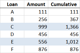
The first 1,000 is reached at loan C. Then, per Anthony’s question, the process would start again at the very next loan. The next 1,000 is reached at loan E, then the process starts again at loan F, and continues.
Now, let’s see how we can have Excel formulas help us out.
Details
As you know, in Excel there are many ways to accomplish any given task. So, this is but one of many possible options. If you have another you’d like to share, please post a comment below.
The approach presented in this post will use two helper columns to define the cumulative range, and then start over when a loan is selected. With these helper columns in place, the selection formula is rather straightforward.
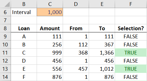
Let’s take a quick look at the end result, and then sort through the details of the formulas:
Let’s take it one formula at a time.
Loan A
From Column: Let’s start with the first loan, Loan A. The initial From value, 1, is just entered into the cell.
To Column: The To formula needs to return the loan amount, 111. One formula to accomplish this is:
=D11+C11-1
Selection Column: The Selection formula needs to return TRUE if the interval value in C6 falls between the From and To values. One way to do this is to use the AND function, which returns TRUE when all of its arguments are TRUE. Something like this would work:
=AND($C$6>=D9,$C$6<=E9)
If the interval value in $C$6 (absolute reference) is both greater than or equal to the From value in D9 (relative reference), and less than or equal to the To value in E9 (relative reference), then the AND function returns TRUE, indicating the loan is selected. Otherwise it returns FALSE, indicating the loan is not a selection.
Now let’s move to the next loan.
Loan B
From Column: The From value for the next loan depends on if the previous loan was selected. If the previous loan was selected, then the From value needs to reset back to 1 because the sampling process begins again. If not, the From value needs to increment the previous loan’s To value by 1. We can use an IF function to accomplish this conditional logic, as follows.
=IF(F9,1,E9+1)
To Column: the logic for the To column doesn’t change from the previous loan, so, we can simply fill the formula from Loan A down.
Selection Column: the logic for the Selection formula doesn’t change from the previous loan, so, we can just fill the Loan A formula down.
Remaining Loans
We can simply fill the formulas for loan B down throughout all remaining loans.
Conditional Formatting
If we wanted to spice things up a bit, we could select the Selection column, and then use the Home > Conditional Formatting > Highlight Cell Rules > Equal To to tell Excel to format the TRUE cells with green or any other preferred format.
Video
I’ve shot a quick video that demonstrates how to write these formulas.
Conclusion
This is but one approach, if you prefer another, please share by posting a comment below!
If you’d like to see the formulas in action, feel free to download the sample file:
Excel is not what it used to be.
You need the Excel Proficiency Roadmap now. Includes 6 steps for a successful journey, 3 things to avoid, and weekly Excel tips.
Want to learn Excel?
Our training programs start at $29 and will help you learn Excel quickly.
Jeff
This was outstanding. Thank you so much for sharing. Love the practical example!
Thanks Dan 🙂
Master Jeff,
Thanks for sharing your expertise with us. I love the way you teach.
another approach for the logic test cell F9 and below: =E11/$C$6>1 turns “true” if the cumulated value in column E exceeds the given level of 1,000
Nice…thanks!
Nice. Thank you Jeff and Carsten.
This is something I use to do using a calculator many years ago. One additional step that I use to do was to take the excess over the given 1,000 and add it to the next amount. Doing this gives a slightly difference results. The formula for D10 would change to =IF(E9>$C$6,E9-$C$6,E9+1). One problem that I noticed in my example is when and amount in Column C is a multiple of the target amount. If this occurred it would require additional formula or manual correction.