Get & Transform: An Alternative to Simple PivotTable Reports
I love PivotTables, and use them all the time. But, when our needs are simple, we can easily summarize data with a Get & Transform query instead. Why? To simplify our workbooks and improve our efficiency. Let me demonstrate.
Objective
Before we dig into the mechanics, let’s just be clear about our goal. Let’s say that each month, we export data from our accounting system into a csv file. Then, we import the csv data into an Excel workbook by doing a copy/paste. Once the transactions are in an Excel workbook, we build a PivotTable report to summarize the transactions. We save the workbook, close, and move on with our life. And life is good … until next period, when we get to do these manual steps all over again.
Instead, we can set up an Excel workbook that will automatically pull in the transactions from the csv file, already summarized! And, it can be updated each month without a single mouse click. That would certainly be faster than the manual way. Is this even possible? Yes, all thanks to Power Query / Get & Transform queries.
I’ve included a short video demonstration as well as all of the detailed steps below for reference.
Video Demonstration
Detailed Steps
Each period, we export transactions from some system, perhaps it is an accounting system, inventory system, AR, AP, ERP, CRM, whatever. The point is that we export transactions as a csv file. In this example, I’ve exported some transactions from my accounting system, and they look a bit like this:
To accomplish our objective, we’ll use these steps:
- Create the Basic Query
- Summarize
- Total Row
- Refresh on Open
Let’s take them one by one.
Note: The steps below are presented with Excel for Windows 2016. If you are using a different version of Excel, please note that the features presented may not be available or you may need to download and install the Power Query Add-in.
Create the Basic Query
First we need to create the basic query. To do this, we click the Data > From Text/CSV command icon from the Get & Transform Data ribbon group.
After browsing to the csv file, Excel provides a quick preview, as shown below.
At this point, we click the Edit button to open the Query Editor, as shown below.
Now, we just need to tell Excel how to summarize the transactions before they are pulled into Excel.
Summarize
Our goal is to summarize the transactions by account, and create one column for each department. There are four steps.
Step 1: Remove Extra Columns. The first step is to remove unnecessary columns, especially those that have unique values in each row, such as the TransID and Date columns. We need to remove them because they will prevent Excel from summarizing the transactions as desired.
In our query, we select the TransID, AcctID, DeptID, and Date columns by holding down Ctrl as we click each column label. Then, we click the Home > Remove Columns ribbon command.
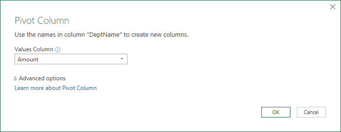
Step 2: Pivot. In order to create one column for each department, we select the DeptName column, and then the Transform > Pivot ribbon command. Excel displays the Pivot Column dialog where we simply identify the values column as Amount, as shown below.
Step 3: Crossfoot. We need to insert a new column that computes the sum of all department values for each account row. To do this, we select all department columns (holding down Shift), and then click the Add Column > Standard > Add command. We now have a new column named Sum, which we can rename if desired by double-clicking the column label or using the gear icon in the applied steps list box.
Step 4: Close & Load. Now, we can click the Home > Close & Load button to send our results back to Excel, as shown below.
Back in Excel, we just have to add a total row.
Total Row
To add a total row, we simply select the results table and then click the Table Tools > Design > Total Row checkbox.
At this point, Excel provides a total row, and sums the final table column. We can easily tell Excel to sum each column by selecting each cell in the total row, and selecting Sum from the drop-down as shown below.
After we do this for each column, our report is complete, as shown below.
Now, the resulting summary table isn’t as flexible as a PivotTable, for example it doesn’t have drill-down, report layout options, or the ability to click-and-drag field items. So, when we need more from a report, we’d want to go with a PivotTable … but … when our needs are simple, this is a nice alternative.
To update this report next period, we would export a new csv file and replace the prior period csv file. That is, we would save it with the name file name to the same folder. (Note: if you want Excel to grab all files in the folder, instead of having to use the same name, consider using the From Folder option instead, as discussed in this post.)
Then, when we open this Excel report workbook, we simply right-click the results table and select Refresh. Excel will retrieve and summarize the contents of the csv file and update our results table. Nice!
Note: If there are new accounts in the csv file, Excel will automatically include them. But, a change to the departments, such as a new department or a removed department, will require an edit to the query in order to ensure the crossfoot column reflects the updated department list.
If we also wanted to eliminate the manual right-click and refresh step, we can tell Excel to automatically refresh the results table when we open the Excel workbook. Here’s how.
Refresh on Open
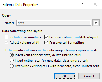
To have Excel automatically refresh the results table when you open the workbook, right-click the results table and select Table > External Data Properties. Excel will display the External Data Properties dialog as shown below.
Next, click the small Query Properties icon on the right side of the Name field to display the Query Properties dialog, as shown below.
Check the Refresh data when opening the file checkbox, and, you should be good to go! Next time you open the Excel file, without any mouse clicks Excel will grab data from the csv file, summarize it, and update the results table. Nice!
Conclusion
If you have any other fun Get & Transform tricks, please share by posting a comment below. And, if you’d like to practice these steps, please download the sample data csv file and give it a try.
Excel is not what it used to be.
You need the Excel Proficiency Roadmap now. Includes 6 steps for a successful journey, 3 things to avoid, and weekly Excel tips.
Want to learn Excel?
Our training programs start at $29 and will help you learn Excel quickly.


Thanks for advising how to automatically refresh a table when opening a workbook (right-click the results table and select Table > External Data Properties, ….
Welcome 🙂
Hullo Jeff,
Wow, you, are amazing as always! You make it so easy!!!
I luv the auto up-date!!!!!
thanks.
Thanks…Glad to help, I LOVE this stuff 🙂