VLOOKUP Hack #2: Range Lookups
In the first VLOOKUP Hacks post, we talked about how the 4th argument impacts the sort order. But, there is more to uncover about this 4th argument. So, let’s pick up right where we left off.
So far, we understand that the 4th argument tells Excel whether we are looking for a value between a range of values or an exact matching value. Its official name is range_lookup, and now it is time to dig into what it actually means.

I have prepared a video demonstration as well as a detailed narrative below for reference.
Video Demonstration
Detailed Narrative
When the 4th argument is TRUE, or omitted, it tells Excel to perform a range lookup. What exactly is a range lookup? It means you are looking for a value between a range of values. The fastest way to explain this is with an example and a picture.
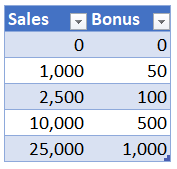
Let’s suppose the sales manager created a sales incentive program for the month. He would like you to pay a bonus amount to the sales reps based on their sales for the month. He then provides you with the following table:

If a salesperson had sales of 1,200 for the month, you would easily find the bonus amount of 50. If a salesperson had sales of 12,345, you would be able to determine the bonus amount is 500.
When you are doing this manually, you aren’t looking for an exact matching sales amount. You are looking for a sales amount that falls between a start and end point.
That is EXACTLY what the 4th argument means! That is a “range lookup.”
So, when the 4th argument is TRUE, you are telling Excel to perform a range lookup. When the 4th argument is FALSE, you are telling Excel to find an exact matching value.
Note: You may see 0 used instead of FALSE in the 4th argument. Excel evaluates 0 as FALSE, and any non-zero number as TRUE.
Now that we have the overall concept down, let’s dig into the Excel details.
Hack
When we humans perform a range lookup, we love seeing both the start and end points. For example, in the sales bonus illustration above, there are From and To columns. Being able to see both sides of the range makes us feel warm and fuzzy. Content. Comfortable.
But, here is the hack: VLOOKUP only needs the From column!
The implications of this are important. So, let’s unpack them. First, here is an updated table that would work perfectly with VLOOKUP:
Here is how I like to think about VLOOKUP. I like to think about it operating in two stages. In stage one, it looks in the first column ONLY. It starts at the top, and goes down one row at a time looking for its matching value. Once it finds it match, then it enters stage two, where it shoots to the right to retrieve the related value.
So, when the 4th argument is TRUE (or omitted), it will look down the Sales column until it finds its row. Any sales amount that is >= 0 and < 1,000 will return a bonus amount of 0. And sales >= 1,000 and < 2,500 will return 50. And so on.
Now that we see how this works, it is easy to understand why the data must be sorted in ascending order when the 4th argument is TRUE. In order for VLOOKUP to return an accurate result when doing a range lookup, the table must be sorted in ascending order by the lookup column. Hopefully, this helps clarify the sort order issue, which we discussed at length in the first VLOOKUP hack post.
Let’s explore this capability with a few examples.
Example 1: Bonus
If we wanted Excel to determine the bonus amount based on sales, we would write the following formula in to cell C7 to retrieve the bonus amount from Table1:
=VLOOKUP(B7,Table1,2,TRUE)
When the sales amount is 12,345, VLOOKUP returns the expected bonus amount of 500, as shown below.

That is the basic operation of range lookups, but, we can apply this in many different ways. For example, we can do a lookup on date values.
Example 2: Fiscal Periods
Fiscal periods…you mean dates? Yes … VLOOKUP can even work with dates! For example, let’s say we need to create fiscal periods based on transaction dates. We could set up a fiscal period table (Table3), like this one:
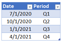
Then, it would be easy to have VLOOKUP retrieve the corresponding quarter label for a set of transactions. For example, we could use VLOOKUP to populate column D shown below.

The formula written into D15 and then filled down, is:
=VLOOKUP(B15,Table3,2,TRUE)
Example 3: Single Column
We can even do a range lookup on a single-column lookup table. This technique provides an easy way to return the beginning point of a range. For example, if we need to find the pay period begin date, we could create a table of pay period begin dates, like this:
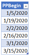
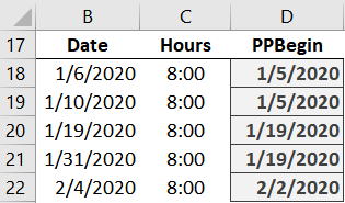
Then, we can use VLOOKUP to return the value from the 1st column of the table (Table4), like this:
=VLOOKUP(B18,Table4,1,TRUE)
We could write the formula into D18 and fill it down, as shown below:
So, that is what it means to perform a range lookup. In the next post, we’ll talk more about the implications of the 4th argument, and how we can use it to help us perform list comparisons, aka, reconciliations!
Excel is not what it used to be.
You need the Excel Proficiency Roadmap now. Includes 6 steps for a successful journey, 3 things to avoid, and weekly Excel tips.
Want to learn Excel?
Our training programs start at $29 and will help you learn Excel quickly.
Thank you so much for this article. I use VLOOKUP all the time but haven’t been taking advantage of the range lookup capability. You’ve saved me at least two hours a month and that’s huge, especially during the month-end and quarter-end reporting rushes!
Welcome! And glad to hear about the time savings, that is what its all about 🙂
A few ideas
A. When I use the VLOOKUP Range based formula I think of it returning the largest pre-defined range value that is less than or equal to the input value.
B. The VLOOKUP Range example for the Sales Incentive situation above can be extended to provide additional capability and flexibility. Consider the following three columns:
1. Trigger X value (E.g. equivalent to the ‘Sales’ column above)
2. Starting Y Value at X (E.g. equivalent to the ‘Bonus’ column above)
3. Incremental Rate (the per X rate that applies after Trigger Value)
The combination of the three columns provides a configurable slope that applies after the trigger X+Y values, instead of just assuming a flat line after the ‘steps’ initial X + Y values.
Assuming the 3 columns above are in Table1, the formula used becomes:
=VLOOKUP(B7,Table1,2,True)+(B7-VLOOKUP(B7,Table1,1,True))*VLOOKUP(B7,Table1,3,True)
E.g. Y at starting point for trigger + (Movement beyond trigger) times Rate after trigger
All kinds of patterns can be concisely setup using that 3 column structure. It can also be translated into SQL database format for user configurable relationships.
Note: I have a template spreadsheet setup that automatically graphs VLOOKUP Range type data onto an XY type graph to help users confirm the values used and highlight potential issues. I cannot attach that here, but can forward a copy on request.
An early use of the three column VLOOKUP Range formula approach above, was also for Sales Incentives.
For that system, the base was not the raw monthly Sales amount, but monthly Sales divided by their Target, that was then mapped to the percentage of Bonus they would be paid.
This is the profile data used:
Trigger, Start, Incremental Rate
0, 0, 0
80, 0, 5 (minimum achievement is 80% after which get 5% more bonus for every 1% extra of target achieved)
100,100,1 (standard is 100% of bonus for achieving 100% of target, then 1% increment per 1%)
120,120,2 (to encourage overachievement, they offered 2% increase per 1% increase in target above 120%)
Visualisation of the pattern via a graph is very useful. Even though Sales Management was warned of the open ended final segment, that pattern was to be used. Then a salesman delayed 3 months worth of monthly sales until the last month of a quarter making them eligible for ~600% of monthly bonus!
Alan … thanks for taking the time to share these wonderful applications of VLOOKUP! Appreciate it!
Thanks
Jeff
Such a simple change ‘False’ to ‘True’ yet so powerful and like Amy’s comments, such a time saver, many thanks for this little gem of information!
Welcome 🙂
I recently came to this Vlookup page from one of your Blog emails. As a 20+ year user of Excel, I first I thought “OK, so here are some entry-level Excel techniques – maybe not much of interest…” but I have to say, your basic walk-through of how Vlookup functions with the “True” argument made me think about Vlookup in a way I hadn’t before. I mostly have used that function to “match” items between tables and to retrieve a specific data element. I had always considered the “True” option to be a handicap, since you could receive a potentially false “match” if your query value wasn’t in the searched table and it would force you to sort your data first. I really hadn’t thought about the utility of using the “True” Vlookup qualifier to select a value (eg. Bonus value) based on a “threshold” (i.e the first value that would meet the criteria – eg. a given sales level), given that Vlookup would trigger on that first value, but rather would likely have written a formula that looked for a value “between” a set of numbers. Often simple is better. Thanks for providing these examples.
But, what if I don’t sort the lookup column?