Unique Data Validation Drop-Down From Duplicate Table Data
In this post, we’ll explore a method for generating a drop-down that contains a unique list of choices derived from a table column with duplicate values.
Objective
Before we get started on the mechanics, let’s take a look at what we are trying to achieve.
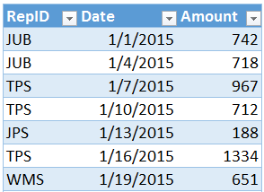
We have a data table that is exported from our accounting system. It contains the rep, the transaction date, and the amount, as shown below.

On another sheet, we want the user to be able to select a rep from a drop-down.
We want the drop-down list to contain a unique list of reps from the table.
The goals for our solution are that it is fast and easy to maintain over time, even when new reps may appear in the data table, that we don’t use VBA macros, that we can move the workbook to other folder locations in future periods, and that we don’t need to update any formulas in future periods.
Ready? Me too…let’s do this thing.
NOTE: An alternative to the technique presented below is to use Power Query instead of a PivotTable as discussed in this post: https://www.excel-university.com/use-power-query-to-create-a-drop-down-list-without-duplicates/
Technique
This technique involves creating a unique list of reps in a worksheet with a PivotTable. The PivotTable is an intermediate step that creates the rep list that we can use to feed the data validation drop-down list. In a way, the data flow for this technique can be visualized as follows:
- Table > PivotTable > Named Reference > Data Validation
Let’s take these steps one at a time.
Table
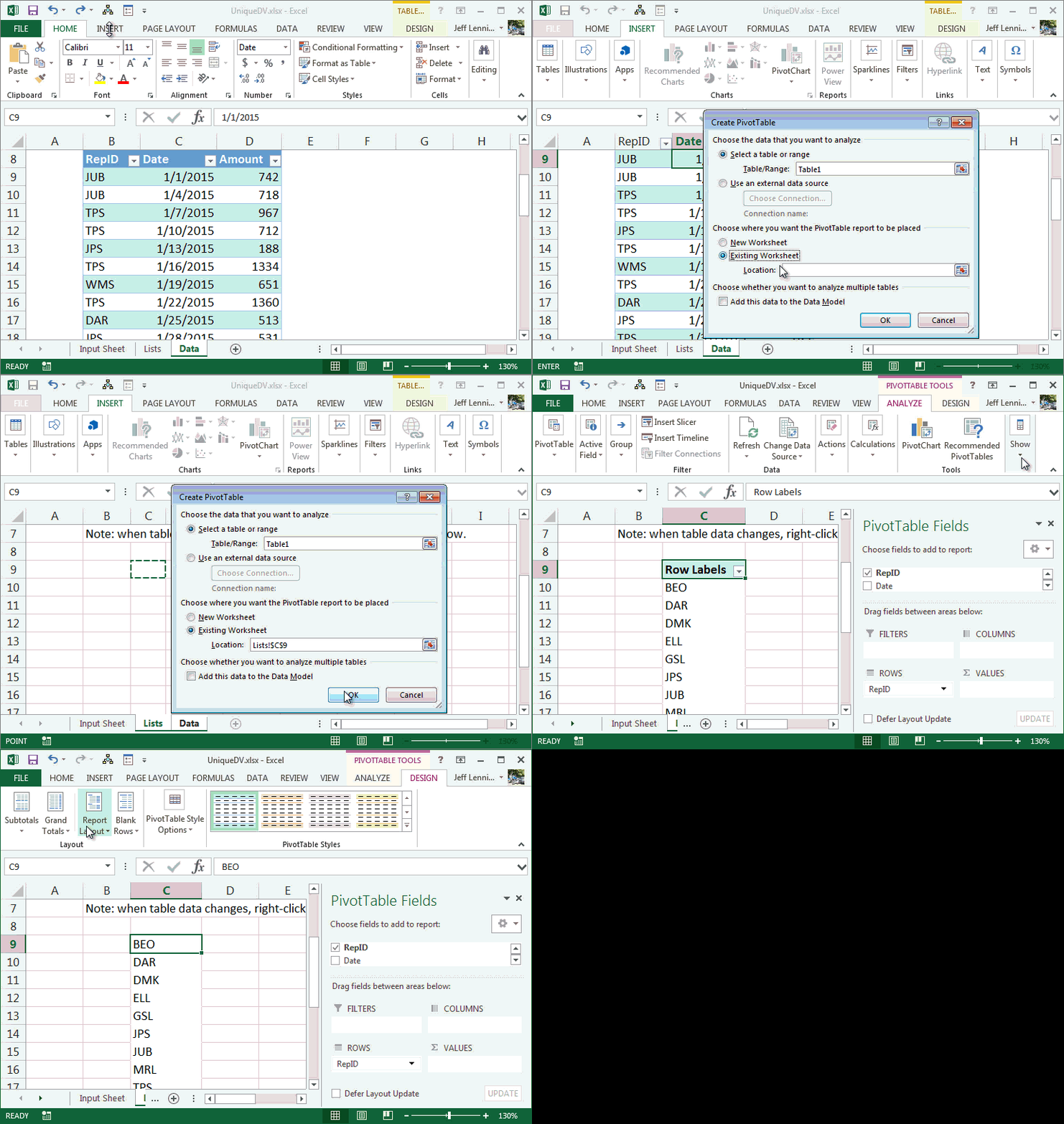
First, we store the source data in a Table. This is easily accomplished by selecting the ordinary range and then the Insert > Table Ribbon icon.
PivotTable
With the table in place, it is time to create the unique list of choices. We select any cell in the table and then the Insert > PivotTable icon. We build a simple PivotTable on a new sheet by placing the field that contains the drop-down choices into the Rows area and removing the field headers and grand totals, as shown below.
Any time you change the underlying table data, such as adding new rows in future periods, you’ll need to update the rep list by clicking the Refresh button (PivotTable Tools > Refresh, or, right-click and Refresh). If you want the list to be sorted as it is refreshed, you can update the sort order of the PivotTable by right-clicking a rep cell and selecting the desired Sort option. If you delete data from the table, and the deleted reps still appear in the PivotTable, head into the PivotTable Options dialog and change the Number of items to retain per field to None.
Now that we have generated a unique list of reps, it is time to put them into a named range that can be used with the data validation feature.
Named Reference
Now, we’ll set up a named range that can be used by the data validation feature to create the drop-down. There are many ways to create a dynamic named range to reference the PivotTable results, and I’ll provide one such solution. If you have any others, please share by posting a comment below.
The named reference needs to dynamically adjust as the number of PivotTable items change. We’ll set up a new name, dd_reps, that uses the following formula:
=Lists!$C$9:INDEX(Lists!$C:$C,MATCH("*",Lists!$C:$C,-1),1)
In summary, this formula creates a range reference that begins with cell C9 on the Lists worksheet (the first cell in the PivotTable) and continues through the cell returned by the INDEX function. The INDEX function dynamically returns the last data cell in column C by using the MATCH function.
To set up the new name, click the New name button in the Name Manager (Formulas > Name Manager) and then enter the name information as shown below.
The resulting name, dd_reps, contains a list of the PivotTable results, even if the number of reps changes over time.
Data Validation
Now, we are home free. All that remains is to set up the drop-down box with the data validation feature (Data > Data Validation).
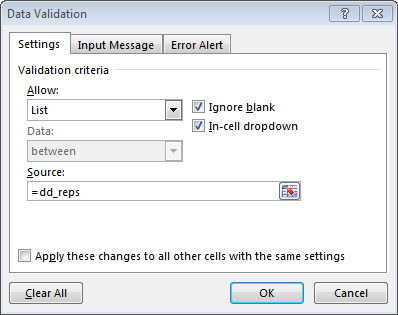
We simply Allow a List equal to the name, dd_reps, as shown below.
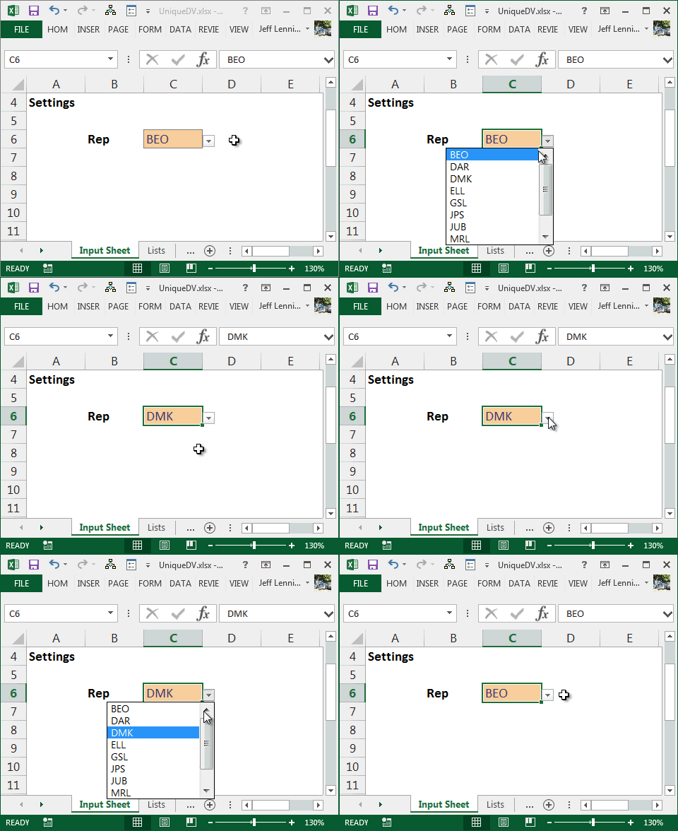
The resulting drop-down contains a list of choices from the PivotTable, as shown below.
Once the workbook is set up, as new data is added to the table each period, you just need to Refresh the PivotTable and any new reps will flow through the PivotTable into the drop-down.
Since this is Excel, there are many ways to accomplish any task, so the method presented above is only one such solution. If you prefer a different solution, we’d love to hear it…please post a comment below and share!
Additional Resources
- Sample File: UniqueDV
- How to do this with Power Query instead of a PivotTable: https://www.excel-university.com/use-power-query-to-create-a-drop-down-list-without-duplicates/
- Posts about Tables
- Posts about PivotTables
- Posts about Data Validation
- Posts about Named References
Excel is not what it used to be.
You need the Excel Proficiency Roadmap now. Includes 6 steps for a successful journey, 3 things to avoid, and weekly Excel tips.
Want to learn Excel?
Our training programs start at $29 and will help you learn Excel quickly.


for validation i used the formula as list
=$C$9:OFFSET($C$9,COUNTA($C$9:$C$100),0,1,1)
I agree I use C100 which means max 100 rows from C9
Venkat,
Thanks for sharing this named reference alternative, which uses the OFFSET/COUNTA combination instead of the INDEX/MATCH combination…thanks!
Thanks
Jeff
I am getting an error when i paste above formula in data validation
Error:
you may not use reference formula or array
You paste the Index formula in to Name Manager not Data Validation.
Very nice! Thanks!
Jeff
Your solution was my first thought but with the users intended to operate this, they couldn’t be relied upon to update the Pivot.
Thanks anyway.
Gary
Gary,
Ah…I see…if you figure out an approach that works for your workbook, please share by posting a comment…thanks!
Thanks
Jeff
Found out a better solution so you don’t have to create a pivot table (if you can include new columns in your database – you can hide everything later):
It will require 3 more columns
Assuming RepID in cell A1; Date cell B1 and Amount cell C1:
1) In column D you will have to exclude duplicated values using IF+IFERROR+VLOOKUP as below:
=IF(A2=IFERROR(VLOOKUP(A2,$A$1:$A1,1,0),””),””,A2)
*** Please note the relative and absolute references carefully
Apply this formula for the whole table
2) In column E you will sum only the values that are shown in column D:
=IF(D2=””,E1,E1+1)
*** In this case the column header must to be empty or equal to zero
Apply this formula for the whole table
3) In column F you will exclude the duplicated numbers:
=IF(E2=E1,””,E2)
Apply this formula for the whole table
4) In another column or sheet (I’ve included in column H of the same sheet):
Include sequential numbers starting by 1 (1, 2, 3, and so on in each line)
You can include as many numbers as you want
5) In column I (in my case) you will lookup the sequential numbers in your table:
=IFERROR(INDEX($D$2:$D$28,MATCH($H2,$F$2:$F$28,0)),””)
Apply this formula for the whole sequence of numbers you created in column H
6) Edit the dd_reps using the new reference:
=Sheet1!G2:INDEX(Sheet1!G:G,MATCH(“*”,Sheet1!G:G,-1),1)
7) Include the validation list with this new sequence
Felipe Maier
Felipe – Thanks for sharing your alternative!
Thanks,
Jeff
I recently did something very similar to Filipe. My slight variation was that if it was the first occurrence (using a similar “if error” reference) and then returned the row(). This gave each first occurrence a unique identifying number. I then used rank() to turn that list of unique but spread numbers into a 1, 2, 3, 4, 5…. On a separate page I had a column of 1, 2, 3, 4, 5, 6, 7 and used it to look up the the row. I think they ways listed here are a bit more elegant, but it is another solution, particularly if you are going to want to make any other references to the list.
I hope this is something excel adds natively in the future. I was recently using Google Sheets and realized that it automatically turns a validation from a duplicated list into an unduplicated drop down. I have to assume an unduplicated list is the goal more often than not.
Thanks!
Thanks for this technique, it was the best one in my search
Welcome 🙂
Hello – I’m digging this method; however, the named range does not appear to be dynamic as expected. It’s only looking at the first cell of the pivot and doesn’t expand when refreshed. My pivot starts at B4 with the Header at B3. Thoughts? Wondering if this method will not work in Excel 2013?
=’Weekly Details’!$B$4:INDEX(‘Weekly Details’!$B:$B,MATCH(“*”,’Weekly Details’!$B:$B,-1),1)
The MATCH * method works on text columns. If you are referencing numeric values instead, you’d want to update it to something like this instead:
MATCH(MIN(B:B)-1,…
Hope this helps!
Thanks
Jeff
Excellent, I will give it a go! That must be it, because it did work on one that is a text column.
Great 🙂
Well, I couldn’t get that to work, so I created another column and formatted the date using TEXT(Week, “Mmm dd yy”) Seems to work ok now. = )
Nice alternative…glad you got it going!
Hi Jeff,
i was thinking about using a pivot table to create a unique list.
Hopefully this is not too long winded but i wasn’t sure how to explain it properly otherwise (so sorry in advance).
I have never coded before recently but have just started and was looking for a guide on how to create dependent data lists with a set up like mine below, eg.,
Expenses Bills Insurance House Contents
Expenses Bills Insurance House Building
Expenses Bills Insurance Car Mine
Expenses Bills Insurance Car Wife’s
Income Mine
Income Wife’s
Income Other
Expenses Shopping General
Expenses Shopping Unecessary
etc.
I want it set up this way so i can add or remove categories without having to create a new validation list for each new category and making sure i add it to all the right columns (my categories go 5 deep so 1 main and 4 dependent).
I could not find anyone with a set up like mine until i came across the following link http://quadexcel.com/create-dependent-drop-down-lists-containing-unique-distinct-values-in-excel/.
It took me about 4 hours (i know next to nothing about formulas – and forgetting to press ctrl+shift+enter half the time and then not properly checking all my cell references…) to apply the formulas & modify for the extra columns i needed to apply them to. I was so happy when i was done but i found that it only worked as long as i did the selection from one cell (for each of the columns required) – i couldn’t have a validation list going down so i couldn’t use it to add data at the end of each column.
I then had to use a macro to add from the second row down to copy it down to the bottom row of the data table. I got this to work 🙂 but i really wanted it to work from a userform, so with more research and help from this link, http://www.contextures.com/exceluserformdependentcomboboxes.html i found i could write the selection back to the spreadsheet for the array formulas to work.
Sorry for the long winded comment. Here is my final formulas
Main list
=IFERROR(INDEX(Type_All,MATCH(0,COUNTIF($J$6:J6,Type_All),0)),””) + ctrl + shift + enter
Second list
=IFERROR(INDEX(SubCat1_All,MATCH(0,COUNTIF($K$6:K6,SubCat1_All)+(Type_All$K$1),0)),””) + ctrl + shift + enter
Third list
=IFERROR(INDEX(SubCat2_All,MATCH(0,COUNTIF($L$6:L6,SubCat2_All)+(Type_All$K$1)+(SubCat1_All$L$1),0)),””) + ctrl + shift + enter
Fourth & Fifth list i just added the extra to the end
The site i got the array formula from was only two lists deep, so with my next to no coding experience i was happy (though not about the four hours) to adjust it to my own lists.
from the user form i have the following code,
Private Sub input6_Change()
Dim ws As Worksheet
Set ws = Sheet2
ws.Range(“k1”).Value = Me.Input6.Value
End Sub
i have done that for each of the combo boxes i have for the independent list – i have called them input6,7,8 etc so i can loop through the adding of data instead of adding each one line by line (i got this tip from http://www.onlinepclearning.com – an efficient coder, trevor easton). Please note the range reference is referenced in the relevant array formula so the lists update automatically and then show in the next combo box.
I don’t know if that might be helpful to anyone else and it is a long winded way to go about it but now i have it set up i can just add my rows of categories and sort them (probably don’t need to sort them but i like them to show in alphabetical order in the drop down lists).
There’s only two other things i would like to do if possible and that if is,
1. remove the zero if from the last columns if they have no categories in them, i.e., if the lists for a particular category are only 3 deep, then the last two drop downs will show a zero in them.
2. i would like to only have the items show in the drop down list and not a whole lot of blank lines below the last unique entry (because my range on the unique list is not dynamic it is a set range), maybe i can play with turning each unique list into a table…
but i find that now my excel hangs and freezes and i can’t get the code to add to the bottom of the data table to work very well, it will work a couple of times and then if i play around with code for anything else not related, it will throw an error with the following line,
Set aNewRow = rng.ListObject.ListRows.Add(AlwaysInsert:=True)
the whole code for adding data is
Private Sub CmdBtn3_Click() ‘Add button
Dim ws As Worksheet
Set ws = Sheet1
Dim inps As Long
Dim rng As Range
Set rng = Sheet1.Range(“ExpensesIncome”)
Dim aNewRow As ListRow
Set aNewRow = rng.ListObject.ListRows.Add(AlwaysInsert:=True)
For inps = 1 To 12
With ws
aNewRow.Range.Cells(1, inps).Value = Me.Controls(“Input” & inps).Value
End With
Next
End Sub
So maybe i have broken my excel with my fancy dependent drop down user form set up 🙁 oh well, it might take me weeks to sort that one out 🙂
Thanks for your time and hopefully it is of help to someone, if you would like more info or better explanation you can email me direct
Cheers
Craig
Works perfectly, thanks!
Can you please explain how the Match portion of the formula is working? How does it give the last cell in the list for the named range?
Power Query is another option – Get and transform from the table – remove all columns save the one of interest – emove rows (remove duplicates) – then load as a table. All that is is required is a refresh if the original table is updated.