Use Power Query to Create a Drop-Down List without Duplicates
In this post, we’ll create a drop-down that contains a unique list of choices derived from a column that contains duplicate values. This may sound familiar as we previously accomplished this with a PivotTable. However, the Power Query feature that’s built-in to Excel 2016 makes this process easier.
Objective
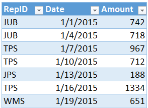
We have a data table that contains RepID, Date, and Amount columns, as shown below.
On another sheet, we want the user to be able to select a rep from a drop-down.

We want the drop-down list to contain a unique list of reps from the table.
Our solution should be fast and easy to maintain over time, even when new reps may appear in the data table. We don’t want to use VBA or to have to update any formulas going forward. Let’s see how Power Query can help.
Steps
We’ll accomplish our objective by performing the following steps:
- Create the query
- Create a name
- Create the drop-down
Well, let’s get to it.
Please note that the steps below are written with Excel 2016 for Windows. If you are using a different version of Excel, Power Query may not be available or you may need to download the free Power Query Add-In.
Create the query
First, we navigate to the worksheet that contains our data table, shown below.
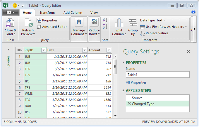
Then, we select any cell within the table and click the following command:
- Data > From Table (in the Get & Transform group)
This launches the Query Editor dialog, as shown below.
The results we want to return should be the RepID column, without duplicates, sorted in ascending order. So, let’s begin by removing the other columns.
With the RepID column selected, we click the following command:
- Manage Columns > Remove Other Columns
The updated query is shown below.

Now, we need to remove duplicates, so, we select the following command:
- Reduce Rows > Remove Duplicates
The updated query is shown below.

Finally, we sort the list in ascending order by using the RepID drop-down. The updated query is shown below.

Last, we need to return the results to Excel, so we use the Close & Load command. Our unique RepID list now appears in a table in our workbook, as shown below.

We are mostly done at this point, and all that remains is to use this list of choices in our drop-down.
Create the name
We need to create a name that refers to the table that stores the query results. There are a couple of options for accomplishing this step. One option is to select all of the data cells in the table, and then enter the desired name into the Name Box (that little box just to the left of the formula bar).
Another option is to use the Name Manager. In order to use the Name Manager, we first need to make a note of the table’s name. To do this, select any cell in the table and then look at the Table Tools > Table Name field. This will show you the current name and allow you to give it a different name if desired. For example, Excel automatically assigned the name Table1_2 to the results table. We could change it if we wanted, but, assuming we don’t, our next step is to open the Name Manager by clicking the following icon:
- Formulas > Name Manager
In the Name Manager dialog, we click the New button to create a new name. We enter the desired name, such as RepList. In the Refers to field, we enter an equal sign and then the table’s name, such as =Table1_2. This is shown below.

We click OK and now that our new name is created, we can set up the drop-down.
Create the drop-down
We select the input cell that should contain our drop-down, and then use the following command:
- Data > Data Validation
In the Data Validation dialog, we want to Allow a List. The Source is equal to our name =RepList, as shown below.

When we click OK, Excel inserts the drop-down, and now we can pick from our list of choices.
Whenever we update the table with new transactions, all we need to do is right-click our results table and select Refresh. Power Query will rebuild the results table, and the values will automatically flow into the drop-down list.
If you have any other fun Power Query ideas, please share by posting a comment below…thanks!
Resources
- Sample file: UniqueDVwithPowerQuery
- Previous post to do this with a PivotTable: https://www.excel-university.com/unique-data-validation-drop-down-from-duplicate-table-data/
Excel is not what it used to be.
You need the Excel Proficiency Roadmap now. Includes 6 steps for a successful journey, 3 things to avoid, and weekly Excel tips.
Want to learn Excel?
Our training programs start at $29 and will help you learn Excel quickly.
This would be useful. Wish it was in Excel 2010.
My friend’s website has installation instructions for 2010, hope it helps: https://www.excelcampus.com/install-power-query/
Thanks
Jeff
How could make multiple drop-down lists that relate to each other so they don’t duplicate selections? For example, if I have a list of tasks with drop boxes containing employee names, how do I prevent the same employee from being selected for multiple tasks?
Boring Task #1 Tom/Jane (drop down list)
Boring Task #2 Tom/Jane (drop down list)
Hey Tristan,
I finally figured it out:) In your situation, you would just have a rule that allows a list, and for the source, you would check the value of the other cell and choose a different value:
=IF(other drop-down=””,dd_list,IF(other drop-down=”Tom”,”Jane”,”Jane”)
And use a similar formula for the other drop-down rule:)
Please let me know if you need further explanations,
Kurt LeBlanc
I’m addicted to your Blog! Keep them coming please!
Will do:-)
I have a question! How do you make a drop down list change formatting on another cell. For example say I have a drop down box of USD and Euro for currency. Then in another column right next to it you want that currency to change with the change of the drop down box. How would you do that? Can you even do that?
Hey Dorothy
Yes:) You can do that using conditional formatting. Use this blog https://www.excel-university.com/excel-conditional-formatting-based-on-another-cell/ from Mr. Jeff, and when you add your own formatting, you can change the number formatting of the cell with the left-most tab. Write your formula and format the number based on the selection.
Let me know how that works!
Kurt LeBlanc
This is ok, but what if I want to create four dependent unique DV lists for filtering table by first DV or 3rd DV or all four DVs ?
Thanks for putting this together! I love how detailed you are, and never skip a step for those of us rookies!
Is there a way to turn this into an image, so I can move it around the screen? I’d like to use it to replace a command box, because I’m having trouble getting the command boxes to activate every time I open the workbook… and I think they are slowing the workbook down.
Thanks again!
Excellent post! I loved it. I have a question, it is possible to make the dropdown to select MULTIPLE values? I would like to have the multiple selected values in a list to filter the report. I’ve already created a list in PQ and used something like Table.SelectRows(#”Changed Type”, each (List.Contains(Selection,[Project Name])=true )).
I need to find a way to populate the List called “Selection” using the dropdown output.
I hope you can guide me