Date Data Validation Drop-Down

In this post, we’ll create two data validation drop-down cells that provide the ability to select From and To dates based on the transaction dates stored in the source data. This will ensure that the date selections fall within a valid range of dates, that is, those months with data in the table. This technique is dynamic, so that as transactions are added or removed, it is easy to update the drop-down lists to reflect valid date choices based on the dates of the transactions.

Objective

Before we dig into the mechanics, let’s review our objective.

We export data from our accounting system on a regular basis, and use it to drive some reports. We’d like to provide the user with the ability to select a From and To date based on the transactions dates.

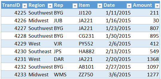
Consider the transaction export below.

Based on the data in the table, we want to provide two drop-downs that allow the user to select a From date and a To date, as follows.

The transactions in the table begin at 1/11/2015. Therefore, we want our From date drop-down to begin with 1/1/2015, and to include the first day of the month for all months with data, such as 2/1/2015 and 3/1/2015. If, next period, the data includes transactions for December 2014, then, we’d like the From date drop-down to include a start date option of 12/1/2014. Same logic for the To date, we want the drop-down to include the last day of the month for all months that have transactions, for example, 1/31/2015, 2/28/2015, and 3/31/2015.

Sound good? Alright, let’s proceed to the mechanics.

Details

To summarize our game plan, we will store the data transactions in a table, create two helper columns in the table that auto-fill as new transactions are added, create an intermediate PivotTable to dynamically provide one row for each From and To date combination, use dynamic named references to grab the PivotTable values, and set up data validation to provide the in-cell drop down.

Let’s proceed one step at a time.

Table

It is very important to store the data transactions in a table (Insert > Table). In this case, it will ensure that any new transactions pasted in future periods will automatically flow through the workbook since tables auto-expand to include new data rows. Plus, tables auto-fill calculated column formulas down…this will ensure that our helper columns automatically fill to any new data rows pasted into the table in the future.

Helper Columns

We’ll create two new helper columns. We’ll be sure to place them to the right of the exported data so that in future periods, we can paste new transactions into the table as they come. Excel will auto-fill the formulas down through the new transactions.

The helper columns will provide the last day of the month and the first day of the month for each transaction date. We’ll name the new columns EOM and BOM for end of month and beginning of month.

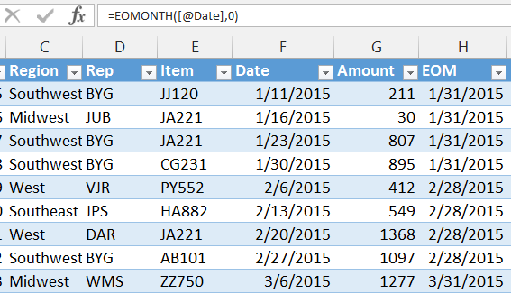
The function that we will use to compute the EOM value is the EOMONTH function. The EOMONTH function is probably my favorite date function, and it returns the last day of the month. It even allows us to add or subtract months so that we can move ahead or back if needed. The formula for the EOM column is:

=EOMONTH([@Date],0)

Where:

• [@Date] is the structured table reference for the current row date column
• 0 is the number of months to add or subtract from the transaction date; 0 since we want the last day of the transaction month

The results are shown below.

We’ll use a similar formula to compute the BOM column. The only twist is that since the EOMONTH function returns the last day of the month, we’ll need to add one day to its result to compute the first day of the next month. So, the formula for the BOM column follows:

=EOMONTH([@Date],-1)+1

Where:

• [@Date] is the date value
• -1 subtracts one month from from the transaction date

The results are shown below.

Since the data is stored in a table, Excel will automatically fill these helper columns down for any new data rows.

PivotTable

With our helper columns in place, it is time to create the PivotTable. The PivotTable will dynamically generate one row for each unique EOM and BOM. We insert the BOM field into the rows area, the EOM field into the rows area, change the report layout to tabular, remove subtotals and grand totals, remove Row Headers formatting, remove the +/- Buttons and Field Headers as shown below.

The PivotTable generates the From and To values that we need. Anytime new transactions are pasted into the table, we can update the PivotTable as needed by clicking the Refresh button (PivotTable Tools > Refresh). Also, we can sort the PivotTable in Ascending order by the BOM field to ensure new report rows appear in chronological order (activate the PivotTable and then use the Home > Sort command).

Named References

Now, we need to set up two named references that we can use in the data validation list source. The names need to dynamically adapt to the PivotTable’s dimensions and increase or decrease accordingly.

There are numerous ways to create a dynamic named range, and I’ll illustrate one such possibility. If you prefer another method, please share by posting a comment below.

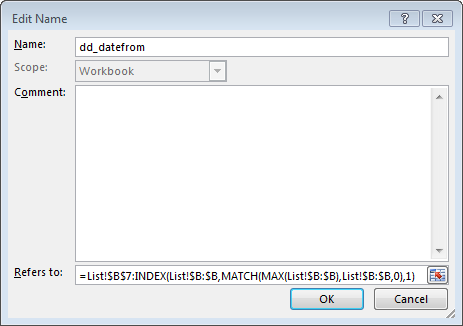
For the From Date column, we’ll use the Name Manager (Formulas > Name Manager) to set up a new name, dd_datefrom. The name will include the range that spans from cell B7 on the Lists worksheet through the last cell in the PivotTable with the following formula:

=List!$B$7:INDEX(List!$B:$B,MATCH(MAX(List!$B:$B),List!$B:$B,0),1)

Where:

• List!$B$7 is the first cell in the range
• INDEX(List!$B:$B,MATCH(MAX(List!$B:$B),List!$B:$B,0),1) determines the last cell in the PivotTable column by returning a cell reference in column B for the max PivotTable value. (Assuming the PivotTable is sorted in ascending order, the max PivotTable value will be the last PivotTable value.) We’ve explored the INDEX and MATCH functions numerous times before, please feel free to reference the related blog posts listed below for additional information.

The screenshot of the name is shown below for reference.

We set up a similar formula for the dd_dateto name, as follows.

=List!$C$7:INDEX(List!$C:$C,MATCH(MAX(List!$C:$C),List!$C:$C,0),1)

With the dynamic names set up, all that remains is to set up the drop-down cells with the data validation feature.

Data Validation

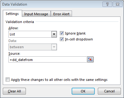
We select the From Date input cell, and use Data Validation (Data > Data Validation) to allow a List equal to the name dd_datefrom, as shown below.

We select the Date To input cell, and set up data validation to allow a list equal to dd_dateto.

Now, the data validation drop down lists contain dates based on the dates in the transaction table as shown below.

As new transactions are added to the table, we simply refresh the intermediate PivotTable to retrieve updated drop-down choices. The dynamic named ranges incorporate them and feed them into the data validation input cells.

Conclusion

There are many ways to accomplish any given task in Excel, so, if you have an alternative or preferred method for any of the steps presented above, please share by posting a comment below…thanks!

Additional Resources

• Sample File: DatesFromTo
• INDEX posts
• MATCH posts