Transpose Values and Formulas in Excel

In this post, we’ll explore three methods for transposing data in Excel. The first method can be used when you just want to quickly to transpose the values manually. The second method can be used when you want formulas to perform the transposition automatically based on the labels. The third method can be applied when you need to frequently paste new transactions and you want them to be automatically included.

Objective

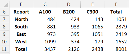
Before we dig into the mechanics, let’s take a quick look at our objective. We exported data from our accounting system, and the extract contains the values we want, but, it is not in the orientation needed for our report. The extract displays regions in rows and items in columns, as shown below:

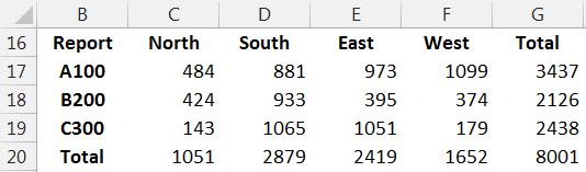
However, for our report, we need regions in columns and items in rows. We need to transpose the orientation, as shown below.

If this is a one-time project, then, we are probably okay to perform this task manually using the Paste Special command.

Paste Special

To perform the transposition manually, we simply select the original range and do a standard copy.

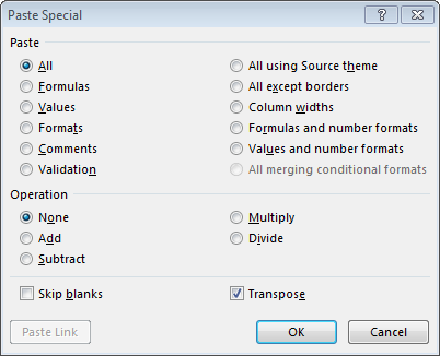
Next, we select Paste Special, and then check the Transpose checkbox in the Paste Special dialog shown below.

Excel transposes the data into the desired orientation.

But, what if this was an ongoing task? For example, maybe we need to transpose the same export on a monthly, weekly, or daily basis. Since we seek to eliminate manual steps from recurring-use workbooks, we’ll delegate the transposition task to Excel formulas.

Transpose with Formulas

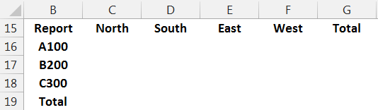
The first step is to get the report labels set up. That means doing a copy, paste special transpose on the report labels. We copy the region labels and paste special transpose. Then we copy the item labels and paste special transpose. The resulting worksheet is shown below.

Now, all that remains is to write a formula that populates the report values. Our goals for the formula are (1) that it will work even if the order of the report labels are different from the order in the data range and (2) that it is consistent within the range. That is, that we can write a single formula, and then fill it down and right throughout the range. We love using consistent formulas because they make the workbook easier to maintain over time. Since this is Excel, there are many ways to handle this. One way it is to use a dynamic SUMIFS function, but, since we have no need to aggregate rows, and we’d like a method that can transpose text as well as numeric values, we’ll use the INDEX/MATCH functions.

The INDEX function returns a value within a range at the intersection of a specified row and column. We’ll use the MATCH function to tell the INDEX function which row and column has the value to return.

First, let me show the screenshot and then explain the mechanics of the formula.

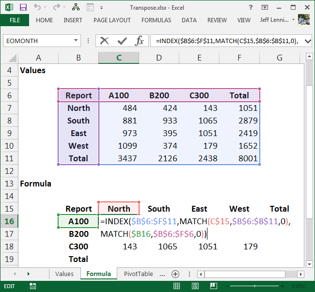
The INDEX function returns a value from a range at the intersection of a given row and column. So, the first argument of the INDEX function is the range from which a value should be returned, in our case, B6:F11. Since we fill the formula down and right, we lock down the range reference with the dollar signs $B$6:$F$11.

The next argument of the INDEX function is row_num, which is the row number that has the value we’d like to return. We ask the MATCH function to figure out the row number. We MATCH the report’s region label, C$15, in the data region column, $B$6:$B$11, and 0 for exact match. Since we fill the formula down and right, we lock down the cell and range references properly. This function provides the row number to the INDEX function.

The next argument of the INDEX function is column_num, which is the column number that has the value we’d like to return. We ask the MATCH function to determine the column number. We MATCH, our report’s item label, $B16, in the data item row, $B$6:$F$6, and 0 for exact match. Since we fill the formula down and right, we lock down the cell and range references accordingly. This function provides the column number to the INDEX function.

The resulting function can be filled down and right throughout the range to successfully transpose the data. Since this transposition was accomplished with a formula, next period, we can simply paste in the updated data and the formula will automatically retrieve the values into the transposed report.

This works great when we are exporting similar data items each period. But, what if the number of rows change each time we do the export? We’ll, this is Excel and there are many ways to handle this, but one nice way is with the PivotTable feature.

PivotTable

The PivotTable feature allows us to generate a report based on a data range.

Since we’ll be adding new transactions each period, we’ll store the underlying data range in a table. This is done the first period by selecting any cell in the range and clicking Insert > Table. The resulting ordinary range has been converted into a table, as shown below.

To create the PivotTable report, we select any cell within the table, and then Insert > PivotTable. In the resulting Create PivotTable dialog show below, we can opt to place the report in a new or existing worksheet, and then click OK.

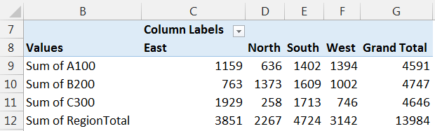
In the PivotTable field list, we insert the Region field into the Columns are by clicking-and-dragging it. We insert the A100, B200, and C300 fields into the report by checking their checkboxes. We then transpose the orientation of the value fields by moving the Values field from the columns are to the rows area. All of these steps are shown below.

If Region totals are needed, we can add a calculated field to the PivotTable. PivotTable Tools > Calculated Field. In the Calculated Field dialog, we would define the name and the formula as shown below.

The resulting transposed report is shown below.

And, the best part is that since tables auto-expand to include any new transactions, we can easily paste in new transactions next period, as shown below.

Back on the PivotTable, we simply right-click and Refresh…the new transactions automatically flow into the report, as shown below.

If we wanted to clean up the report, we can rename the report labels, apply number formatting to the value fields, and click-and-drag the region columns into the desired order.

Conclusion

In Excel, it seems there are many ways to accomplish any given task. The above methods happen to be my preferred ways to transpose data. If you have any other methods for transposing data, we’d love to hear about it…please share by posting a comment below.

Additional Resources

• Sample file: Transpose
• Other INDEX posts
• Other MATCH posts
• Dynamic SUMIFS Post
• Other Table posts
• Transpose with a Get & Transform query