Perform Lookups with FILTER 1

This is the first post in a series where we’ll talk about how to use the FILTER function as an alternative to lookup functions including VLOOKUP. Why? Well, as we’ll discover in this series, the FILTER function offers several key benefits. For example, FILTER supports:

• Multiple return columns
• Multiple lookup columns
• Multiple matching row values

In this first post, we’ll see how the FILTER function can return multiple column values. This is much different from VLOOKUP which is designed to return a value from a single column.

Return Multiple Column Values

Before we get too far, let’s just confirm the Excel scenario we are trying to tackle.

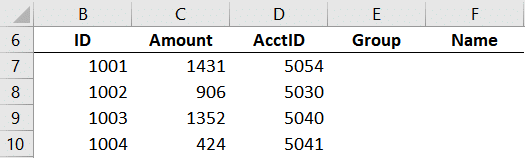
We have some transactions, like this:

We need to retrieve the account names and groups from a lookup table like this:

One option would be to use a traditional lookup function such as VLOOKUP. In this case, we would write two formulas, one to retrieve the Name and another to retrieve the Group. And that would be fine. In fact, this is a common method we’ve used for decades. But, now we have another option. The FILTER function can return multiple columns. This means that we can write one formula instead of two (or more) to retrieve multiple column values.

Note: depending on your version of Excel, you may not have access to the FILTER function. At the time of this writing, it is available in Excel 365.

Details

The FILTER function is designed to return a subset of data, meaning, selected rows (or columns) from a data table. The basic syntax is this:

=FILTER(array, include, [if_empty])

Where:

• array is the range you wish to filter
• include is the expression that defines which rows/columns to retrieve
• [if_empty] is an optional value to return if no items are found

So, Jeff … that doesn’t really sound like a lookup function. I know. And so often, when an Excel user is presented with a lookup task, traditional lookup functions such as VLOOKUP immediately come to mind. But, sometimes, there are alternatives to VLOOKUP which provide some benefits.

Note: other examples include SUMIFS and Power Query.

So, let’s see how we can apply the FILTER function to accomplish our lookup task.

Illustration

We want to write a formula in E7 to populate both the Name and Group values.

That formula should retrieve values from C15:D23 by finding a matching AcctID in B15:B23 here:

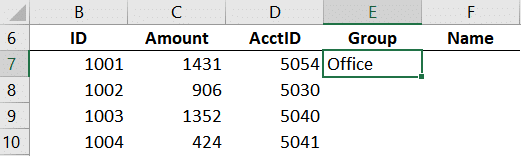
So, in cell E7, we write the following formula:

=FILTER($C$15:$D$23,$B$15:$B$23=D7)

We hit Enter … and bam:

That one formula returns both the Name and Group values … yay!

We can fill the formula in E7 down to populate the remaining transactions:

In this illustration, the column order was the same … Name and then Group. But … what if the column orders are different? No problem.

What if the column order is different?

Let’s say the column order is different. For example, Group then Name in one place:

And Name then Group in another:

One way to accomplish this is to FILTER a FILTER. In other words, we use FILTER to retrieve all columns that match the AcctID like we did previously with this formula:

=FILTER($C$15:$D$23,$B$15:$B$23=D7)

And then FILTER those results to only include one column. We can tell the FILTER function which column we want based on matching the column labels.

We wrap another FILTER function around the previous FILTER function and use the include argument to compare the column labels in C14:D14 with the column label in E6. We are careful to use the proper absolute/relative references so that when we fill down/right it continues to work as expected:

=FILTER(FILTER($C$15:$D$23,$B$15:$B$23=$D7),$C$14:$D$14=E$6)

We hit Enter and bam …

Now, we can fill that formula down and right … and bam:

Yay … we did it!

Conclusion

As you can see, the FILTER function provides an alternative to traditional lookup functions such as VLOOKUP. One benefit is that it supports multiple return columns … which is another way to say it can return multiple values from related columns.

In the next post, we’ll talk about how the FILTER function supports multiple lookup columns.

In the meantime, let me know what you think about the FILTER function by writing a comment below … thanks!

Sample file: