Perform Lookups with FILTER 2

This is the second post in a series where we are talking about how FILTER can be a nice alternative to traditional lookup functions such as VLOOKUP.

In the first post, we saw how the FILTER function supports multiple return columns (it can return values from multiple columns). In this post, we’ll see how the FILTER function supports multiple lookup columns (multiple lookup values).

Note: depending on your version of Excel, you may not have access to the FILTER function. At the time of this writing, it is available in Excel 365.

Multiple Lookup Columns

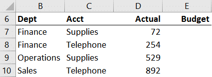
Before we dive into the mechanics, let’s just step back and confirm our objective. We have exported some expense totals from our accounting system, like this:

We want to retrieve the Budget amount from our budget table (Table1) which looks like this:

The key observation here is that there isn’t a single lookup column. To find our matching budget value requires us to consider multiple values … Dept and Acct.

With a traditional lookup function such as VLOOKUP, we would first need to combine the Dept and Acct labels in order to create a single lookup column. After all, VLOOKUP is designed to operate on a single lookup value. And that would be fine. This is how we’ve been approaching this issue for decades.

But, if we use FILTER instead of VLOOKUP, we wouldn’t need to combine multiple columns to create a single lookup column. FILTER can operate on multiple lookup columns. Let’s check it out.

Details

The FILTER function has the following arguments:

=FILTER(array, include, [if_empty])

In the first post, we used a single condition with the include argument. Now it is time to use multiple conditions with the include argument.

We need to understand how to express multiple conditions in a single argument. In summary, we wrap each condition in parentheses and combine them with an operator to express AND or OR logic.

To start, let’s test for a single condition. To test if ColumnA is equal to ValueA, we would use this logic in our include argument:

(ColumnA=ValueA)

Let’s say we also wanted to test if ColumnB is equal to ValueB. If both conditions need to be true, this is AND logic which is expressed with a multiplication operator * like this:

(ColumnA=ValueA)*(ColumnB=ValueB)

If instead only one condition needs to be true, this is OR logic …which is expressed with the addition operator + like this:

(ColumnA=ValueA)+(ColumnB=ValueB)

Now that we see how to write a single include argument that tests for multiple conditions, let’s put this knowledge to use and complete our objective.

Illustration

Table1 contains the budget values we’d like to retrieve:

We want to pull them into the Budget column of our summary:

So, in E7 we write the following:

=FILTER(Table1[Budget],(Table1[Dept]=B7)*(Table1[Acct]=C7))

We hit Enter and bam …

We fill the formula down … and got it!

Now the great news here is that we were able to work with the data as it comes, rather than having to first combine multiple lookup columns as we’ve done for decades with VLOOKUP. So, as you can see FILTER can be a nice alternative to VLOOKUP in some cases.

What do you think about FILTER? I’d love to know … post a comment below to share your thoughts.

Sample File