VLOOKUP on Multiple Columns and Return Text

You want to perform a lookup with VLOOKUP, but, there are multiple lookup columns. So, what are you supposed to do? Combine them into a single lookup column? That is certainly one option, but, as with just about anything in Excel, there are multiple ways. In a previous post, I showed one way to do this with SUMIFS when the value you want to return is a number. In this post, I’ll demonstrate how to return text values when there are multiple lookup columns using a Get & Transform query.

Objective

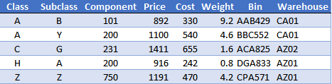
Before we get too far, let’s clarify our objective. We have two systems that store inventory information. Unfortunately, there isn’t a unique ID code that is shared between the two systems. But, there are three columns that together provide the unique identifier, specifically, the Class, Subclass, and Component columns as shown in Table1 below.

We need to retrieve related values from another system based on these three columns. An example of the export from the second system shown in Table2 below.

To perform such a task with VLOOKUP, we would first need to combine, or concatenate, the three lookup columns into a single column. So, instead of that, we’ll see how a Get & Transform query (Power Query) enables us to work with the data as it comes. I’ve created a video along with a detailed narrative for reference.

Video

Details

We’ll walk through this process one step at a time, as follows:

• Connect to Tables
• Merge Tables
• Load Results

Let’s do it!

Note: The steps below are presented with Excel for Windows 2016. If you are using a different version of Excel, please note that the features presented may not be available or you may need to download and install the Power Query Add-in.

Connect to Tables

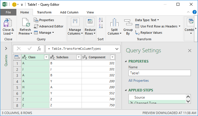
The first step is to get the table data loaded into the Query Editor. This is done by selecting any cell in the first table, Table1, and then selecting the Data > From Table/Range command found in the Get & Transform ribbon group. The table data is loaded into the Query Editor as shown below.

Since we have no transformations, we can simply use the Close & Load To … command, and select Only Create Connection, as shown below.

We do the same steps for our second table, Table2.

With our two tables loaded into Power Query, it is time to merge them.

Merge Tables

This is the step that essentially performs the lookup (instead of VLOOKUP). We begin by selecting the Data > Get Data > Combine Queries > Merge command.

In the resulting Merge dialog, we select our first table, Table1, and then our second table, Table2, as shown below.

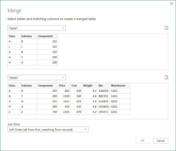
Now, here is the key step. We need to tell Excel how these tables are related. In a typical scenario, there is a single column that we can select in both tables. But, in our scenario, there are three columns we need to select.

Our goal here is to select the three lookup columns in Table1 and then select the related columns in Table2 IN THE SAME ORDER. I don’t mean that the columns need to be positioned in the same order, like Class first, then Subclass, then Component. I mean you have to SELECT them in the same order, even if they are arranged in a different order within the table.

We can do this by holding down either the Shift key or Ctrl key while clicking the columns. If they are arranged next to each other as above, we can click the first column, hold down Shift, and then click the last column. Or, we can independently select columns one at a time by holding down Ctrl while clicking. When done, Excel indicates the order by putting a little 1, 2, and 3 in the column headers. The 1, 2, and 3 need to represent the same columns in both tables, as shown below.

We click OK, and we see the results in the Query Editor, as shown below.

The final step is to identify which fields from Table2 we want to return. To do this, we click the expand columns icon on the right side of the Table2 header, or, select the Table2 column and use the Transform > Structured Column > Expand command.

We simply check the boxes for the columns we want to include. In our case, we want the Price, Bin, and Warehouse columns. The results are shown below.

With the hard work done, it is simply time to load the results to Excel.

Load Results

To load the results back to our Excel workbook, we just use the Home > Close & Load To… command. We opt to send the results back to a Table either in a new or existing worksheet. And bam … multicolumn lookup complete!

And look, not a VLOOKUP or concatenation formula anywhere to be found 🙂

Now, next period, all we need to do is right-click the results table and select Refresh. Any new or updated values in Table1 or Table2 are immediately reflected in the results table. Nice!

The sample file is included below for reference in case you’d like to check it out.

Sample File: MultipleColumns.xlsx