PivotTable Calendar
Excel has numerous date-related features and functions. In this post, we’ll explore a few of them. We need an illustration that will tie them all together, so, we’ll create a graphical calendar with a PivotTable. Even if you don’t need a graphical calendar in your workbooks, the underlying mechanics that enable us to build it can be used in many other situations.
Objective
Here is what we want to build:

This is a graphical PivotTable calendar. We can pick the desired month from the filter control, and the PivotTable updates accordingly.
To build this, we’ll need to explore a few functions, specifically, we’ll use: TEXT, WEEKNUM, and DAY.
I’ve created a video and narrative with the details below.
This post is brought to you by Excel FSM. Before we jump to the details, I’d like to thank our sponsor Excel FSM. Excel FSM (Financial Statement Module) is a patented Excel add-in that enables accountants to more easily create financial statements from a trial balance (or many trial balances to prepare consolidated financials).
It allows you to work with any system that can export a trial balance file. And if you or your clients are using QuickBooks, Excel FSM transforms Excel into a financial statement writer for QuickBooks.
The Excel add-in allows you to define the report groups and create the reports. Updating the financials going forward is just a matter of exporting an updated trial balance and hitting refresh.
If it sounds like Excel FSM could help save you some time, get more information and a free trial here:
Thanks again to Excel FSM for sponsoring this post!
Video
Narrative
We’ll walk through this process using the following steps:
- Date Table
- Basic PivotTable
- PivotTable Formatting
Let’s get to it.
Date Table
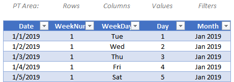
The first step is to build a table that stores the dates for the periods you want to display in your calendar. I’ll show the completed table first, and then we’ll walk through the formula for each column. At the end of the day, we need one column for each PivotTable layout area (Rows, Columns, Values, Filters). So, to help visualize where these columns will end up in the PT, I’ve noted them in the screenshot below:
WeekNum Column: To compute the WeekNum column, we can use the WEEKNUM function and use the value in the Date column as its argument, as shown below:
=WEEKNUM([@Date])
The WEEKENUM function returns the week number of the date. We’ll use this value to create our PivotTable rows.
WeekDay Column: To compute the WeekDay column, we’ll use the TEXT function which returns a text value with the specified formatting. The formatting we’ll use in this case is “ddd” which returns the three-letter abbreviation. (You could also display the day name fully spelled out with “dddd.”)
=TEXT([@Date],"ddd")
We’ll use this column to create our PivotTable columns.
Day Column: To compute the Day column, we can use the DAY function which returns the day number of the date:
=DAY([@Date])
We’ll use this column to create our PivotTable values.
Month Column: To compute the Month column, we can use the TEXT function again, but with different formatting codes:
=TEXT([@Date],"mmm yyyy")
The “mmm yyyy” format code tells Excel we want a three-letter month abbreviation and a 4-digit year. You could use other codes as desired, for example “mmmm” would be the month name fully spelled out and “m” would be the month number.
We’ll use this column to create our PivotTable filters.
With our date table complete, it is time to create our basic PivotTable.
Basic PivotTable
To get our basic PivotTable created, we just select any cell in the Date table and select Insert > PivotTable. We can place the PT on a new or existing sheet.
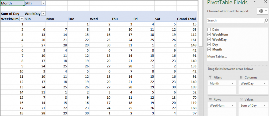
We click and drag to insert the WeekNum field into the Rows layout area, the WeekDay field to the Columns area, the Day field to the Values area, and the Month field to the Filters area. We should see something like this:
And believe it or not, our basic PivotTable is done! Now, it is just a matter of formatting.
PivotTable Formatting
First, we’ll ask Excel to preserve the current column widths. To do this, we select PivotTable Tools > Options. In the resulting PivotTable Options dialog, we uncheck the Autofit column widths on update checkbox.
Remove Grand Totals: Next up, we want to remove grand totals. So, we click PivotTable Tools > Grand Totals > Off for Rows and Columns.
Filter: Next, instead of showing all of the months, we can just pick a single month using the Month filter drop-down. I’ll pick Jan 2019, and at this point we are looking pretty good:
We’ll apply a few more cosmetic things to clean it a little more.
Field Headers: we’ll remove the field headers by toggling off the PivotTable Tools > Field Headers command.
Banding: we check the PivotTable Tools > Banded Rows and Banded Columns checkboxes.
PivotTable Style: we’ll pick any style we like from the PivotTable Tools > Styles gallery. I picked “Light Blue, Pivot Style Dark 2.”
Hide WeekNum column: if you want to hide the WeekNum column, just right-click that worksheet column label (B, C, D, …) and select Hide from the shortcut menu.
And, I think we got it!

Feel free to download the working sample file: PivotTableCalendar.xlsx
If you have any other fun date, calendar, or PivotTable tips, please share by posting a comment below … thanks!
Disclosures and Notes
- This is a sponsored post for Excel FSM. All opinions are my own. Excel FSM is not affiliated with nor endorses any other products or services mentioned.
- 100% of sponsor proceeds fund the Excel University scholarship and financial aid programs … thank you!
- If you’d like information on becoming a sponsor, please check out our sponsorship opportunities page.
Excel is not what it used to be.
You need the Excel Proficiency Roadmap now. Includes 6 steps for a successful journey, 3 things to avoid, and weekly Excel tips.
Want to learn Excel?
Our training programs start at $29 and will help you learn Excel quickly.


Does the pivot table video cover how to put months in the order you want? We have providers whose fiscal year begins differently. The pivot table always put January first. Is there a way to go July, August, September, etc. OR October, November, December, etc.?
Although the video in this post doesn’t cover that, I’d probably create a fiscal period lookup table to reference. That way, I could use either a formula or Power Pivot to sort by the fiscal periods (rather than the calendar periods). One example of creating a fiscal period lookup table is here, and it may help to get your started:
https://www.excel-university.com/create-fiscal-year-periods-with-vlookup/
Thanks
Jeff
Jeff,
Loving this Pivot Table calendar – this will make generating calendars much less cumbersome.
Question: Can event info by date be added easily.
i.e. on Jan calendar
25th day – Dinner with the neighbours
26th day – Gym @ 6 am
Feb
3rd day – Read at Sunday services
etc…
Thanks,
John
Thanks John!
Regarding adding events … that may be a great topic for an upcoming blog post, thanks!
Thanks
Jeff
I second that request for more info on adding event info to certain dates…i hope a blog on that topic does get posted!
Thanks!
Kyle
Very simple, very very good, thanks Jeff
I love this calendar apart from one little problem. When I create the Pivot table my days start at Monday, this means that in December my first week dates (Monday to Sunday) show as 2,3,4,5,6,7,1 Any idea how to change this?
Hi Jane,
You can change the order of PivotTable columns in a couple different ways. One way would be to click-and-drag the column label cells to the desired order (eg, Sunday to Saturday). Or, another way is to type Sunday into the cell that currently says Monday. (Or, Sun if you are using three-letter abbreviations). When you type something into a PT column label cell, if you use the exact text as an existing column label, the order will be updated. But, careful, because if you enter a text value that is not a current column label, then Excel will rename the column label (instead of moving it).
Hope this helps!
Thanks
Jeff
A pivot table would not have been my first thought to create a calendar, but this is quite quick and easy. I have one question on the filter. In the sample file the choices in the filter drop down are in date order but in the video they are alphabetized. What do you need to do to get the filter order that is in the sample file?
Hi Jeff,
I need to reference a cell that has the number of the week within a given month. Can the date table help me do that?