Excel Month List

In this post, we’ll create a list of months with a single Excel formula. To make it more interesting, we’ll allow the user to enter the desired number of months to display and create additional formulas to show the last day of each month, the number of days in the each month, the month number, the year, and a formatted monthly label. Let’s get started.

Objective – Excel List of Months

Before we get too far, let’s confirm our goal.

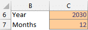
We would like the user to enter the year and the desired number of months, like this:

And we would like Excel to update our list of months accordingly:

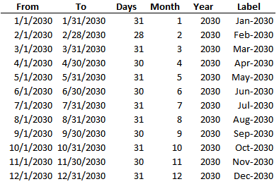
When the user changes the year or the number of months to be displayed, we want Excel to update it automatically.

Note: not all versions of Excel contain all functions presented below.

Video – Excel Month List Formulas

If you prefer to watch a video for the steps on how to create a month list in Excel:

Written Narrative – Excel Month List

In this written narrative, we’ll create one formula for each column in our Excel month list. Let’s just take them one at a time.

To write our formulas, we’ll need to note the location of the Year and Months input cells (C6 and C7):

Let’s start by writing a formula to populate the From column.

From Column

To populate the From column, we’ll use the DATE and SEQUENCE functions.

The DATE function creates a date value for a given year, month, and day. For example, DATE(2030,1,1) would create a date that corresponds to January 1, 2030.

In our worksheet, we want to retrieve the year value entered by the user in C6, so we could use this formula:

=DATE(C6,1,1)

When we hit Enter, we get a single date value.

But, what we’d really like is for Excel to create multiple date values. Specifically, it should create the number of dates specified by the user in C7. For this, we can use the SEQUENCE function.

In summary, the SEQUENCE function creates a sequence of values, such as 1, 2, 3, 4, 5 and so on. We can use the SEQUENCE function as the month argument of the DATE function, like this:

=DATE(C6, SEQUENCE(C7), 1)

We hit Enter, and bam:

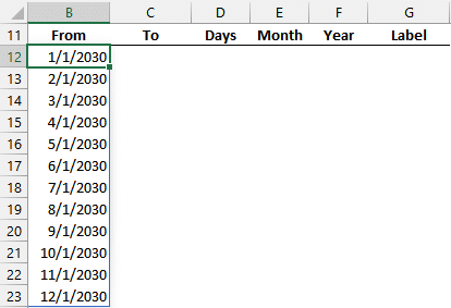
Note: if you see the date serial values instead of formatted dates, just apply a date format to the column.

To Column

We can use the same DATE and SEQUENCE functions to generate the To column, which needs to display the last day of the month.

Let’s start with the DATE function again.

There’s a cool trick to know about the DATE function … you can use 0 for the day to return the last day of the prior month. For example, DATE(2030,1,1) would return January 1, 2030 whereas DATE(2030,1,0) would return the day before that, or December 31, 2029.

We can use that to our advantage here to compute the last day of each month. The only twist is that we will need our SEQUENCE function to start at 2 instead of the default of 1. We can define this start value in the third argument of the SEQUENCE function.

So, our formula in C12 would be this:

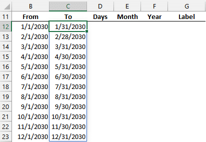
=DATE(C6, SEQUENCE(C7,,2), 0)

We hit Enter, and bam:

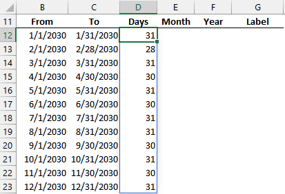
Days Column

In this case, a fairly easy way to compute the number of days in the month is by looking at the day number of the last day of the month in column C.

The DAY function returns the day number of any date value. So, we can use the following formula in D12:

=DAY(C12)

However, when we hit Enter, the formula does not spill down the range like the first two formulas. No worries, we can append the spill reference operator (#) to our cell reference C12 like this:

=DAY(C12#)

Now we hit Enter, and bam:

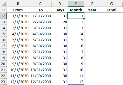
Month Column

To compute the Month column, we can use the MONTH function which returns the month number of any date value. We can reference the date value in either column B or C as desired. We’ll need to be sure to use the spill reference operator so that Excel fills the formula down, like this:

=MONTH(B12#)

We hit Enter, and bam:

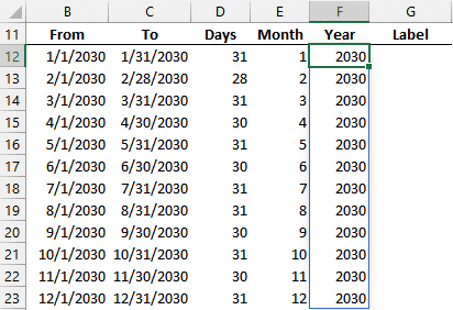
Year Column

The Year column can be computed using the YEAR function, like this:

=YEAR(B12#)

And Bam:

Label Column

For the Label column, we can use the TEXT function to display a date value in our desired format. For example, the format code “mmm” would display the three-letter month abbreviation. The format code “mmmm” would display the month name fully spelled out. The format code “mmm yyyy” would display the three-letter month abbreviation along with a four digit year. The many format code options are documented in the Excel help system in case you’d like to explore others.

In our case, we’ll use the following formula in G12:

=TEXT(B12#,"mmm-yyyy")

We hit Enter and bam:

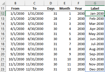
Yay … we did it!

And, if the user enters a different year or number of months, Excel instantly updates the worksheet accordingly.

Conclusion

If you have any questions about the functions used, please let me know in the comments section. Also, if you have any alternatives or suggestions to improve the formulas, please share by posting a comment below … thanks!

Sample file