WRAPROWS WRAPCOLS

Sometimes when we copy data into Excel—from websites, reports, or bank statements—it doesn’t arrive in a nice, neat table. Instead, it comes in as one long line of values, either in a row or a column. That’s where WRAPROWS and WRAPCOLS come in.

Video

Tutorial

In this post, we’ll explore how to use these functions to transform a linear list into a table-like shape—great for readability, structure, and analysis. We’ll also see how these pair beautifully with TOCOL and TOROW, depending on the situation.

---

What is WRAPROWS?

WRAPROWS Function Returns: A reshaped array that wraps a single row or column of values into multiple rows (like breaking a long list into shorter rows).

Syntax:

WRAPROWS(vector, wrap_count, [pad_with])

• vector – The original list of values (a single row or column)
• wrap_count – Number of values per row
• pad_with – (Optional) Value to use if there aren’t enough values to fill the last row

---

Exercise 1: Wrapping a List into Rows

In the Exercise 1 worksheet, we’ve got a simple list of values in a single column (a “vector”). Let’s say we want to display these in multiple rows, wrapping every few values.

Try this:

Formula in cell E6:

=WRAPROWS(B7:B14, 4)

This will take the 8 values and wrap them every 4 values, giving us a 2-row table:

Want to change the number of values per row? Just tweak the wrap_count.

For two values per row:

=WRAPROWS(B7:B14, 2)

But what if we use a wrap_count that doesn’t divide evenly—like 3?

=WRAPROWS(B7:B14, 3)

This results in an error in the last cell because there aren’t enough values to complete that final row:

To handle that, we use the pad_with argument.

Padding the Last Row

You can pad the leftover cells with:

• A zero → =WRAPROWS(B7:B14, 3, 0)
• A dash → =WRAPROWS(B7:B14, 3, "-")
• Or even leave it empty → =WRAPROWS(B7:B14, 3, "")

---

What is WRAPCOLS?

WRAPCOLS Function Returns: A reshaped array that wraps a single list into columns—going top-to-bottom before moving left-to-right.

Syntax:

WRAPCOLS(vector, wrap_count, [pad_with])

• vector – A one-dimensional list (row or column)
• wrap_count – Number of values per column
• pad_with – (Optional) Filler for missing values

---

Wrapping a List into Columns

Still in Exercise 1, try this:

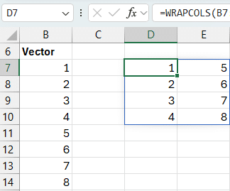
Formula in cell E15:

=WRAPCOLS(B7:B14, 4)

Now the data wraps down first, then moves right into a new column:

And just like WRAPROWS, if the final group is incomplete, you can pad it.

=WRAPCOLS(B7:B14, 3, "")

---

Exercise 2: Cleaning Up a Copy-Paste Mess

In Exercise 2, we simulate a real-life scenario: you copy a list of bank transactions from a website or PDF, and instead of a nice table, it pastes into one single column.

Each transaction actually includes 3 elements:

• Date
• Amount
• Description

They just all end up in one long column like this:

We want to get one row per transaction.

Enter: WRAPROWS

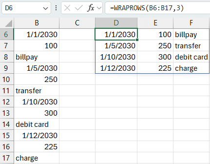
Formula in cell D6:

=WRAPROWS(B6:B17, 3)

This tells Excel:

• Wrap every 3 values into a row
• That gives us 3 columns: Date, Amount, Description

And now we’ve got a clean, structured table again:

Pro tip: If the date column doesn’t look like a date, it might just need formatting. Apply a date format and you’re good to go.

---

Exercise 3: Wrapping More Complex Transaction Data

Let’s level it up.

In Exercise 3, we’ve got more detailed transactions. Each transaction includes:

• Date
• Amount
• Category
• Description

Again, it’s all been dumped into a single column.

To reshape it:

Formula in cell D6:

=WRAPROWS(B6:B21, 4)

This wraps every 4 values into a single row—giving us one clean row per transaction with all the fields:

---

Bonus: Reversing It with TOCOL

What if we want to go the other way—take a nicely structured table and flatten it back into a single column?

That’s where TOCOL comes in.

TOCOL Function Returns: A single-column array from a multi-row, multi-column range.

Formula in cell I6:

=TOCOL(D6#)

And just like that, the transaction table is flattened back into a vertical list:

TOCOL is the inverse of WRAPROWS
TOROW is the inverse of WRAPCOLS

---

Conclusion

If you’ve ever pasted messy data into Excel—or wanted to reshape a list into a table—WRAPROWS and WRAPCOLS can save the day. These functions help you go from chaos to clarity with just a formula or two.

Pair them with TOCOL or TOROW for even more control when flattening or re-wrapping your data.

As always, let us know in the comments if you’ve used these in creative ways—or if you have any questions about getting them to work in your own files!

Sample File

You can download the Excel file here to follow along with all three exercises. It includes the original pasted data, wrapped results, and TOCOL examples.

Requires Excel 365 or Excel 2021+ for WRAPROWS, WRAPCOLS, TOCOL

---

FAQ

1. What’s the difference between WRAPROWS and WRAPCOLS?
WRAPROWS wraps data across rows (left to right), while WRAPCOLS wraps it down columns (top to bottom).

2. When should I use pad_with?
Use pad_with when your data doesn’t divide evenly—like wrapping 8 items into groups of 3. It fills any missing values.

3. What’s a “vector” in Excel?
A vector is just a single row or single column of values. Both WRAPROWS and WRAPCOLS require a one-dimensional list.

4. How is this different from TRANSPOSE?
TRANSPOSE flips rows and columns, but it doesn’t allow you to control how many values per row/column like WRAPROWS does.

5. Can I combine WRAPROWS with TOCOL?
Yes! Use TOCOL to flatten a range, then wrap it using WRAPROWS if you need to change the layout again.

6. My wrapped values are showing as numbers instead of dates. What do I do?
Apply a date format to those cells—Excel stores dates as serial numbers, but formatting makes them readable.

7. Do WRAPROWS and WRAPCOLS work with dynamic arrays?
Yes! They fully support dynamic arrays and will automatically expand if your source range grows.