TOROW TOCOL

When we’re working with structured data in Excel—especially data that comes in from reports or exports—it’s not always in the best shape for analysis. Sometimes, the data we receive is cross-tabulated (months as columns, categories as rows), but we need it in a flat format.

Video

---

Tutorial

In this tutorial, we’ll explore two powerful Excel functions—TOCOL and TOROW—that help reshape data. Then we’ll take it a step further and unpivot the data using a clever formula trick. Finally, we’ll wrap it up by creating a quick summary using the PIVOTBY function.

Understanding the TOCOL Function

TOCOL Function Returns: A single-column array by flattening values from a range or array.

Syntax:

TOCOL(array, [ignore], [scan_by_column])

• array – The range of values to flatten
• ignore – (Optional) Specify if blanks, errors, or both should be ignored
• scan_by_column – (Optional) TRUE to scan down columns first; default is FALSE (scans rows first)

---

Exercise 1: Flattening a Range to a Single Column

In the Exercise 1 worksheet, we have a small matrix: three categories (Rent, Utilities, Phone) across three months (Jan, Feb, Mar). This kind of data layout is common in cross-tabbed reports.

Default Flattening (Row-by-Row)

To flatten this into a single column:

Formula in cell G7:

=TOCOL(C7:E9)

This gives you all the values in one column:

By default, TOCOL goes left to right (row-wise), then down.

Column-by-Column Flattening

If you want the column-first scan (i.e., top-down for each column), just set the third argument to TRUE.

Updated Formula:

=TOCOL(C7:E9,,TRUE)

Now the result reads down each column before moving right:

---

Understanding the TOROW Function

TOROW Function Returns: A single-row array by flattening values from a range or array.

Syntax:

TOROW(array, [ignore], [scan_by_column])

• array – The range to flatten
• ignore – (Optional) Skip blanks, errors, or both
• scan_by_column – (Optional) TRUE to scan down columns first

---

Creating a Flattened Row

In the same worksheet, try:

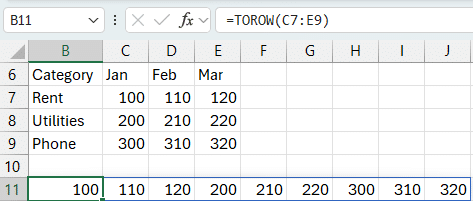
Formula in cell B11:

=TOROW(C7:E9)

This gives you all values across a single row:

Want to scan top-to-bottom down each column first? Just set the last argument to TRUE.

Formula:

=TOROW(C7:E9,,TRUE)

---

Exercise 2: Using TOCOL for an Unpivot

We’ve now got the tools to tackle a common data transformation: unpivoting.

In Exercise 2, we’re working with a similar matrix of values, and we want to flatten it into a format with Month and Amount columns.

Step 1: Flatten the Amounts

Simple enough—just apply TOCOL to the value range.

Formula in cell G7:

=TOCOL(C7:E9)

Step 2: Repeat the Month Labels

Here’s the challenge: we want the month labels (Jan, Feb, Mar) repeated down for each category. TOCOL alone won’t do that, but we can use a trick with IF.

We’ll use the fact that any non-zero number is treated as TRUE in Excel’s calculation engine.

Formula in cell F7:

=TOCOL(IF(C7:E9,B6:D6))

Let’s break this down:

• IF(C7:E9,B6:D6) – If the value is non-zero, return the month label.
• TOCOL(...) – Flatten the result into a single column.

Now we have a matching list of months aligned with the amounts:

---

Handling Zero Values

What if one of the values in your data is 0? In our earlier trick, Excel treats 0 as FALSE, and skips that label.

To fix that, we update the IF function to check for non-blank values instead:

Updated Formula:

=TOCOL(IF(C7:E9<>"",B6:D6))

Now the month label shows up even when the amount is zero.

---

Exercise 3: Full Unpivot with Category, Month, and Amount

Now let’s go all the way: we want to unpivot this cross-tab into a flat list with three columns—Category, Month, and Amount.

Here’s how we do it step by step:

---

Step 1: Category Column

Use the same logic as before. We want to repeat each category (from column B) for every month.

Formula in cell G7:

=TOCOL(IF(C7:E9,B7:B9))

This gives us:

Step 2: Month Column

Repeat the month headers for every value:

Formula in cell H7:

=TOCOL(IF(C7:E9,C6:E6))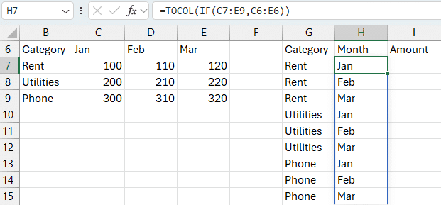

Step 3: Amount Column

This one’s easy—just flatten the data:

Formula in cell I7:

=TOCOL(C7:E9)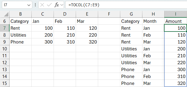

Together, these three columns represent the unpivoted version of the original matrix—perfect for use in PivotTables, charts, or Power Query.

---

Bonus: Create a Summary with PIVOTBY

We unpivoted the data—now let’s pivot it back using Excel’s PIVOTBY function to summarize amounts by category and month.

PIVOTBY Function Returns: A summarized array (like a pivot table) based on specified row and column fields.

Syntax:

PIVOTBY(row_fields, column_fields, values, function)

• row_fields – The field(s) to group by rows
• column_fields – The field(s) to group by columns
• values – The values to aggregate
• function – The aggregation function (e.g., “SUM”)

Formula in cell K6:

=PIVOTBY(G7#,H7#,I7#,SUM)

This gives you a clean, compact pivot-style summary that:

• Auto-includes total rows and columns
• Summarizes the data by category and month
• Doesn’t require a separate PivotTable object

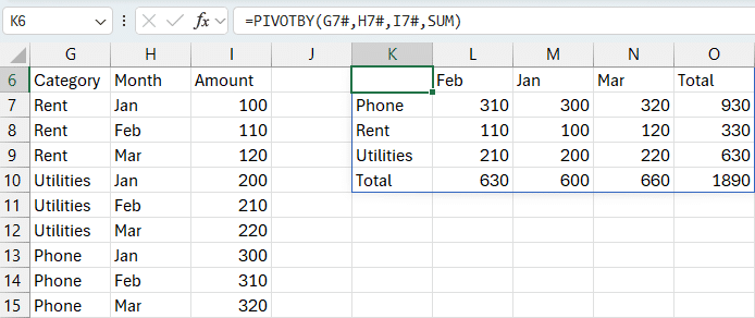
The result is a dynamic pivot table built entirely with formulas.

---

Sample File

You can download the sample workbook here to follow along with the exercises. Each worksheet (Exercise 1–3) demonstrates a key use of TOCOL, TOROW, and unpivoting tricks.

Note: These functions are available in Excel 365 and Excel 2021+.

---

Conclusion

The TOCOL and TOROW functions give you powerful new ways to flatten and reshape your data in Excel. With a bit of creativity—like using the IF function to repeat headers—you can build full unpivot transformations right in your workbook.

And when you’re ready to summarize, PIVOTBY lets you create pivot-style reports without even using a PivotTable.

Whether you’re cleaning up a one-time report or building dynamic dashboards, these tools can make your Excel work faster, cleaner, and more flexible.

Got questions or tips of your own? Drop them in the comments—we’d love to hear how you’re using these functions in your work!

FAQ

1. What’s the difference between TOCOL and TOROW?
TOCOL flattens a range into a column, while TOROW flattens it into a row. Both accept optional arguments to control how they scan data.

2. Why does TOCOL skip zeros in my IF formula?
Zeros are treated as FALSE in logical tests. Use <>"" in your condition to avoid skipping valid zeros.

3. Can I ignore blanks or errors using TOCOL or TOROW?
Yes. Use the second argument (ignore). For example, =TOCOL(range,1) will ignore blanks.

4. How do I manually repeat column or row labels in an unpivot?
Use IF together with TOCOL. For example, =TOCOL(IF(data_range<>"", header_range)).

5. Can I use these functions with Excel Tables?
Yes! You can reference structured Table columns just like regular ranges.

6. What if my data changes in size?
Using Excel Tables helps keep formulas dynamic. TOCOL and TOROW will expand with the table if you reference it correctly.

7. Is PIVOTBY the same as a PivotTable?
PIVOTBY mimics a PivotTable, but works entirely with formulas. It’s great for creating summaries without inserting PivotTable objects.