Get & Transform: An Alternative to Reformat Macros

Excel 2016 includes a set of features called Get & Transform. In previous versions of Excel, these capabilities were included in the Power Query Add-In. In this post, we’ll see how a Get & Transform Query can be used as an alternative to a VBA macro.

Overview

Here is the scenario. We export data out of some system, and save it in a CSV file. We then need to prepare it for use. Perhaps to import into another system, or perhaps to use in a PivotTable or formula-based report. We basically need to clean up the data, remove some columns, change the headers, and so on.

Back in the old days, we could automate such a task with a VBA macro that reformatted the data. Yes, it was difficult to write initially, but, it felt great when we got it working. And life was good, until something in the data changed….like a new column. Some type of change like this could break the macro. Then, we would need to crack open the Visual Basic Editor and troubleshoot. It took some time to figure out how to resolve the issue, but, it felt great once we got it working again. Until something else changed. Argh.

The good news is that a Get & Transform Query is an easy alternative to building such a VBA macro. Best of all, modifications are easy to make when something changes.

Objective

For the purposes of this post, here is what we’d like to automate without a VBA macro:

• Retrieve data into Excel from a CSV file
• Put all email addresses into lower case
• Put all state codes into UPPER case
• Capitalize the first word of all other names
• Remove a column
• Order the columns
• Change the column headers
• Filter out certain rows

And, we want to be able to refresh next month with a single click, or better yet, no click.

Sound like a tall order? It is easy these days. All we need is a Get & Transform Query.

Note: if you are working along in a version of Excel other than Excel 2016 for Windows, you may not have the Get & Transform tools, or, you may need to download the Power Query add-in.

Details

Let’s just jump right in. We’ll basically take the steps in the same order as the bullets above.

Retrieve CSV data

We’ll retrieve orders from a CSV file that was exported from our ecommerce system. But, if you are working with data in some other format, you’ll be glad to know that Get & Transform works with tons of data sources.

Note: if you’d like to work along with these steps, feel free to download the sample data file using the link at the end of this post.

To begin, we create a new workbook and then select the following Ribbon command:

• Data > New Query > From File > From CSV

This opens the Import Data dialog, where we simply browse to and select the CSV file. Once we do, we are presented with a dialog that allows us to preview a sample of the data, as shown below.

Since our data needs to be cleaned up a bit, we’ll click the Edit button. This opens the Query Editor dialog, as shown below.

Now, it is time to clean up, or transform, our data.

Before we jump in, it is important to realize that the following transformations are done inside of Excel, and are not being made to the source data. The source data, in our case the CSV file, is left unaltered. The preview just shows what our data will look like when it arrives in Excel.

Lower case

The first task is to clean up the email address column. Since the customers enter their information online, the email addresses are inconsistent. Some customers enter their address in all caps ([email protected]), some in lower case ([email protected]), and some in proper case ([email protected]). Since we like our data to be nice and tidy, we’ll convert all email addresses into lower case. To do so, we begin by selecting the email column as shown below.

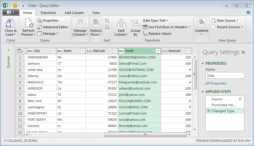
To transform into lower case, we can either right-click the column header and select Transform > lowercase, or, click the following Ribbon icon:

• Text Columns > Format > lowercase

Either way, Excel updates the data as shown below.

Note: to undo a step in the Query Editor, you click the corresponding x in the Applied Steps list box.

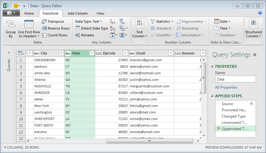
Upper case

Also sloppy is the State code. We have upper, lower, and mixed case. So, we right-click the State column header, and transform to UPPERCASE. The results are shown below.

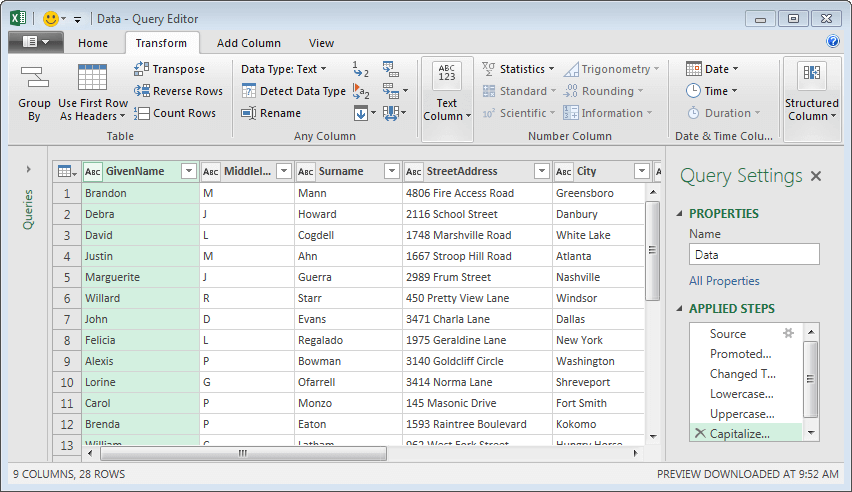
Capitalize

Actually, the City, StreetAddress, GiveName, and Surname columns are all sloppy as well. So, we simply transform each of them to Capitalize Each Word. The clean results are shown below.

Remove columns

We don’t need the MiddleName column, so, we’ll remove it. We can do it with the Remove Columns Ribbon command, or, we can simply right-click the column header and select Remove.

The update is shown below.

Order the columns

We need to change the order of the columns. To do so, we can just click-and-drag the column headers, or, right-click a column header and use the Move option.

In our case, we need the email address column to be the first column, so, we just right-click the Email column header, and select Move > To Beginning.

The update is shown below.

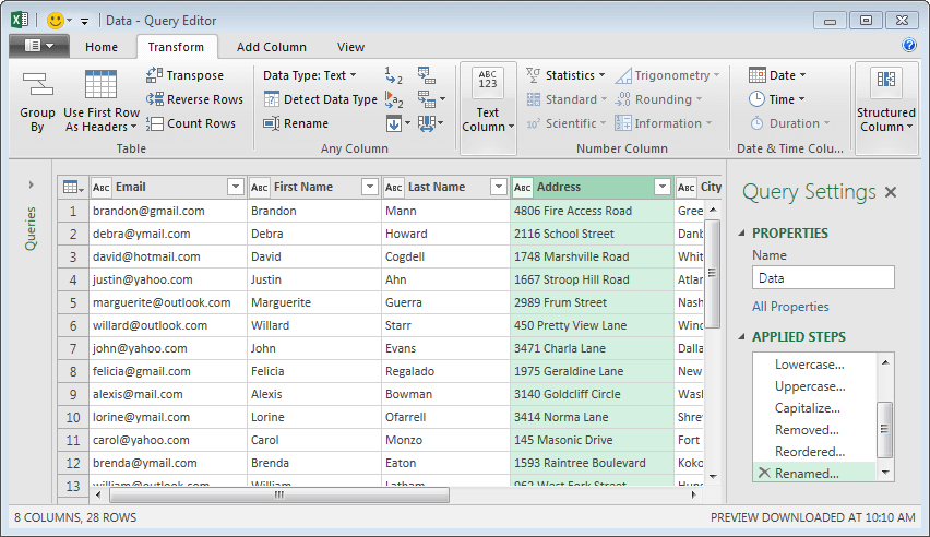
Change column headers

Now we’d like to update the column headers. Doing so is straightforward. We can right-click the column header and select Rename, or, use the following Ribbon command:

• Transform > Rename

We update the GivenName header to First Name, Surname to Last Name, and StreetAddress to Address. These updates are shown below.

Filter

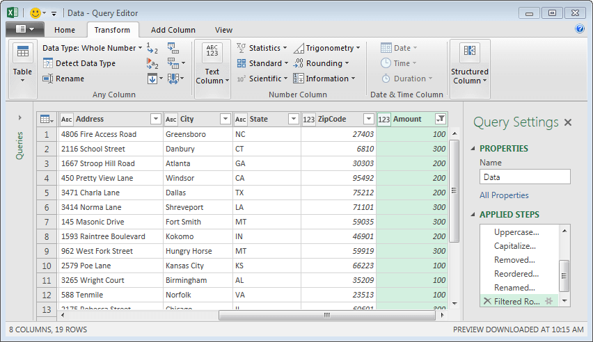
Finally, we want to exclude any rows where the amount is zero. To do this, we simply select the drop-down in the Amount column header, and select Number Filters > Does Not Equal…0.

The update is shown below.

With our data cleaned up and looking good, we are ready to bring it into Excel.

Load

To return the data to Excel, we use the Close & Load command. If we have a specific destination in mind, such as existing worksheet, we can click Close & Load To. If we just want to pull the data into a new worksheet, we can click Close & Load. In our case, we click Close & Load, and bam…the transformed data flows into an Excel table as shown below.

And…we didn’t use a single line of VBA code to do it!

Updating

What about updating next period? Well, it is easy. There are actually two issues to consider. The first is updating the Excel file with newly exported CSV data. The second is updating the query to perform different steps. Let’s talk about both issues.

New Data

When you export new data next period, if you save it in the same folder and with the same file name as the old CSV, all you need to do in Excel is right-click any data cell and select Refresh, or, use the following Ribbon command:

• Query Tools > Refresh

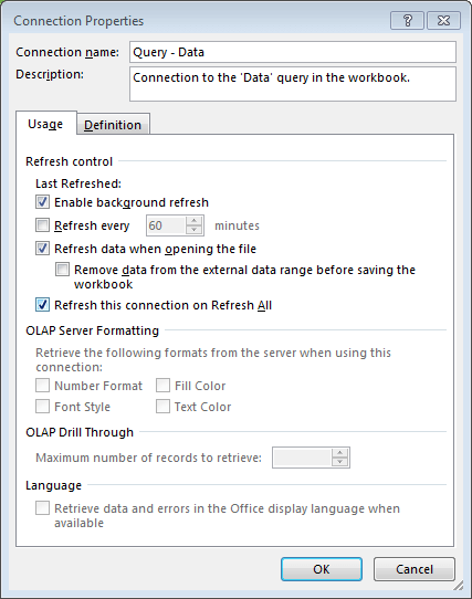
That will update the table with a single click. Can you have Excel update the data without any clicks? Yes, you can ask Excel to refresh the query automatically when you open the workbook. To do this, right-click any data cell, and select Table > External Data Properties. In the resulting External Data Properties dialog, click the little Connection Properties icon to the right of the Name field. In the resulting Connection Properties dialog, check the Refresh data when opening the file checkbox, as shown below.

Now, you just export the new CSV file, save it to the same folder with the same name, and then open your Excel file. Excel will automatically apply the transformations and retrieve the updated data into the table. Wow.

If you use a different file name, then you’ll need to edit the query. Which also happens to be how you add, edit, or delete steps. So, let’s talk about how to edit the query.

Edit the Query

To edit the query, you can select any data cell and then double-click the query in the Workbook Queries panel, or, click the following Ribbon command:

• Query Tools > Edit

This will display the Query Editor dialog. Here, you can change all kinds of things. To edit an existing step, click the gear in the Applied Step panel. For example, to change the data source, click the gear on the Source applied step. To change the order of a step, right-click it and select Move Up or Move Down.

To delete a step, click the x in the Applied Step dialog.

To add a new step, select the last step and then perform the task. To add a step in the middle of the current steps, select any step and then perform the task. Be careful when inserting an intermediate step because it may affect subsequent steps and break your query.

Conclusion

If you haven’t yet played with the Get & Transform features, they are worth digging in to. I don’t want to sound overly dramatic here, but, they are a game changer. They provide us new ways to solve old issues and allow us to easily accomplish tasks that were previously really hard or impractical. I have a series of Get & Transform blog posts topics lined up that will demonstrate some of the capabilities. If you have any Get & Transform tips, please share by posting a comment below…thanks!

Additional Resources

• If you’d like to practice the steps above, open a new Excel workbook and then use this sample CSV data file: Data