VSTACK HSTACK

Ever find yourself combining data from multiple reports—maybe quarterly exports or regional summaries? If you’ve been manually copy-pasting data together, it’s time to meet your new best friends: VSTACK and HSTACK.

Video

---

Tutorial

These two functions make it easy to stack datasets vertically or horizontally without breaking a sweat. In this post, we’ll explore both functions using a few simple examples from our workbook, and show you how to use them to streamline your data prep.

Understanding the VSTACK Function

VSTACK Function Returns: An array where multiple ranges or arrays are stacked on top of each other vertically (like appending rows).

Syntax:

VSTACK(array1, [array2], …)

• array1, array2, … – Ranges or arrays you want to stack on top of each other

---

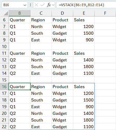
Exercise 1: Combining Quarterly Exports with VSTACK

In the Exercise 1 worksheet, imagine we receive Q1 and Q2 sales data from different sources. These could be on different sheets or files, but for simplicity, they’re side by side.

We want to combine them into one list. Here’s how to do it:

Formula in cell E6:

=VSTACK(B6:E9, B12:E14)

This stacks:

• Q1 data (which includes column headers)
• Q2 data (without column headers, since they’re already in Q1)

And the result is a vertically combined list that’s ready for analysis:

Think of VSTACK like appending rows. It works best when both ranges have matching column structures.

---

Understanding the HSTACK Function

HSTACK Function Returns: An array where multiple ranges or arrays are stacked side-by-side (horizontally, like adding new columns).

Syntax:

HSTACK(array1, [array2], …)

• array1, array2, … – Ranges or arrays you want to place side-by-side

---

Exercise 2: Combining Regional Sales Horizontally with HSTACK

Sometimes, you don’t want to append rows—you want to compare data side-by-side.

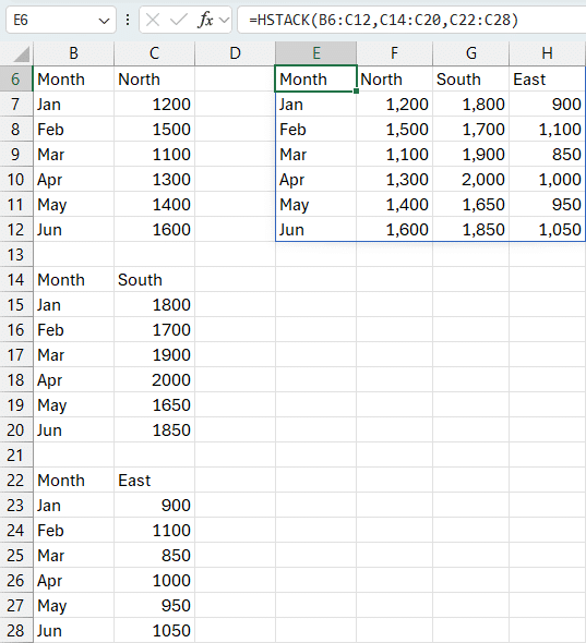
In the Exercise 2 worksheet, we have monthly sales data for three regions: North, South, and East. Each region has its own column of sales figures.

To place all this together in a single table:

Formula in cell B6:

=HSTACK(A6:A10, B6:B10, C6:C10)

Here’s what we’re doing:

• A6:A10 → Month names
• B6:B10 → North region sales
• C6:C10 → South region sales

We already have the month names in column A, so we don’t need to repeat them from each region’s data.

You’ll get a clean table with months and all three regional sales figures lined up horizontally:

Adding a Total Row

Want a total for each region? Just use Alt + = on the cells below to insert the SUM function automatically.

Pro tip: You can label the row “Total” and apply cell formatting for a polished report.

---

Manually Typing Arrays with VSTACK

Sometimes you don’t have column headers in your data—or maybe you want to add your own custom headers manually. No problem. VSTACK can handle that too.

Let’s check out Exercise 3.

Example: Adding Manual Headers with VSTACK

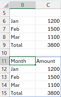
In this exercise, we want to add column headers above our data using manually typed text.

Formula in cell E6:

=VSTACK({"Month","Amount"}, B6:C9)

Results:

Here’s what’s happening:

• {"Month","Amount"} is a manually typed array with two text values
• B6:C9 contains the actual data
• VSTACK puts the custom headers on top of the data

The key here is the use of curly braces {} to define a horizontal array.

This trick is great when you’re building custom summaries or dashboards where headers aren’t present in the source data—or when you want to override them.

---

Conclusion

The VSTACK and HSTACK functions open up a new world of flexibility in Excel. Whether you’re combining exports, comparing regions, or building dashboards, these functions help you organize your data without manual work.

We can now cleanly and dynamically stack datasets vertically or horizontally—and even build custom arrays with headers on the fly.

Give these functions a try in your next report. And as always, if you have questions or creative ways you’ve used them, drop a comment—we’d love to hear from you!

Sample File

You can download the sample Excel workbook here to follow along with all exercises. Each worksheet is labeled (Exercise 1, 2, 3) and matches the examples in this post.

Make sure you’re using Excel 365 or Excel 2021+ to access the VSTACK and HSTACK functions.

---

FAQ

1. What version of Excel supports VSTACK and HSTACK?
These functions are available in Excel 365 and Excel 2021 or later.

2. Can I stack more than two ranges with VSTACK or HSTACK?
Yes! Both functions can take multiple arrays, like =VSTACK(array1, array2, array3).

3. Do the columns have to match when using VSTACK?
It’s best if they do—VSTACK doesn’t align columns by header; it just stacks the arrays as-is.

4. What happens if I include column headers in both arrays when using VSTACK?
You’ll get duplicate headers. Usually, include headers only in the first array.

5. Can I use these functions with data from other worksheets or workbooks?
Absolutely. You can reference ranges from any worksheet or even external workbooks.

6. Can I use HSTACK with different numbers of rows?
Yes, but the shorter arrays will fill with #N/A to match the height of the tallest array.

7. How do I manually type arrays into VSTACK or HSTACK?
Use curly braces {} and separate elements with commas (for horizontal arrays) or semicolons (for vertical arrays).

8. Can I sort or filter the result of a stacked array?
Yes! You can wrap the result in functions like SORT or FILTER to further analyze the data.

---