Split Amount into Annual Columns

Hello and welcome to our guide on how to split amounts into annual columns! We will tackle this using a built-in tool called Power Query. If you’ve never used Power Query in Excel before, no worries, I’ll guide you through the process one step at a time!

Video

Objective

We are trying to split a table of amounts, like this:

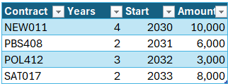
Into annual columns, like this:

This tutorial demonstrates how to accomplish this with Power Query so that it is easy to refresh when there are new contracts added.

Tutorial

Let’s walk through this process by exploring three exercises.

Exercise 1: Setting Up Power Query

We have several contracts which span numerous years, and we want to allocate these into annual columns. We’ll start by using Power Query, a built-in Excel feature that can handle this task efficiently.

Step 1: Load Data into Power Query

Select your data range: Select any cell within the source data table.

Load data into Power Query: Go to the Data tab and select From Table/Range. This action opens the Power Query Editor.

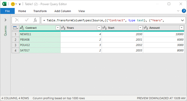
Step 2: Calculate the Annual Amount

• Select the Amount column.
• Hold down Ctrl and then click the Years column.
• Go to Add Column, then Standard, and choose Divide.
• Rename the new column Annual Amount by double-clicking the column header and entering the new name.

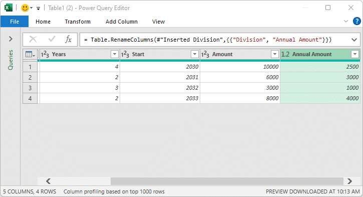
Now that we have the Annual Amount to display in each year column, it is time to take the next step.

Exercise 2: Insert Rows for Each Year

Next, we need to copy the Annual Amount value into yearly columns based on the contract terms. Before we create a column for each year, we’ll create a new row for each year. Later, we’ll move the row values into separate year columns.

Add a Custom Column for Years

Add Column: Click Add Column and then Custom Column.

In the resulting dialog, we want to give the column a name, such as Year. Then, we’ll enter the following formula in order to create a list of years beginning at the Start year and ending the specified number of years later:

= { [Start] .. [Start] + [Years] - 1 }

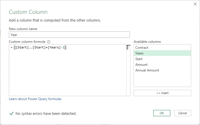
Click OK to see the new Years column filled with lists of years.

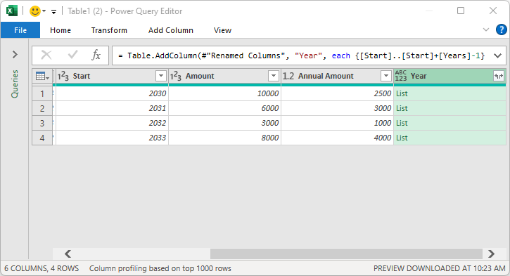
Expand the Custom Column

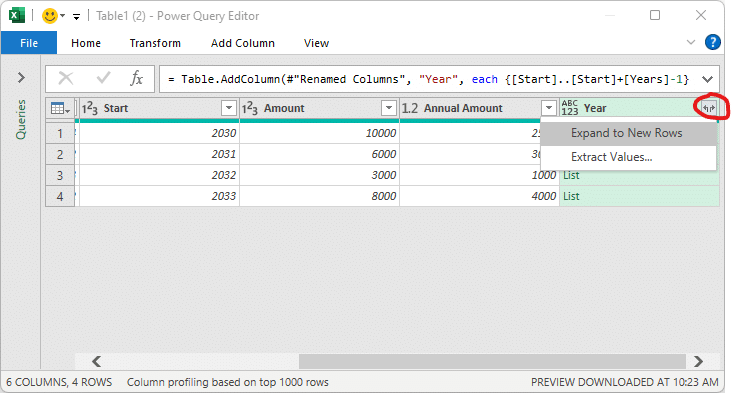
Now we need to tell Power Query to expand the Year column in order to create one row for each Year in the list. We can do this by clicking the small icon next to the Year column header and selecting Expand to New Rows.

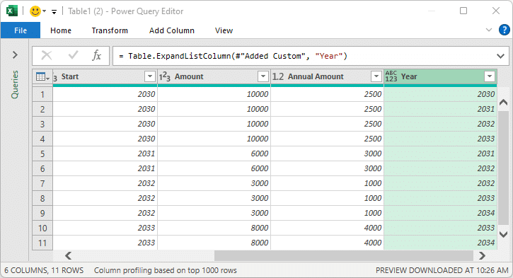
Now we have one new row for each year, and all values have been filled into the new rows:

The final step is to somehow convert these year rows into separate year columns. We’ll do that in the final exercise.

Exercise 3: Pivot the Year Column

In the final exercise, we will pivot the Year column to create annual columns.

Select the Year column, go to Transform, and choose Pivot Column.

Set the Values Column to Annual Amount.

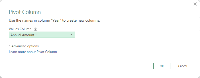
Click OK to see the pivoted columns.

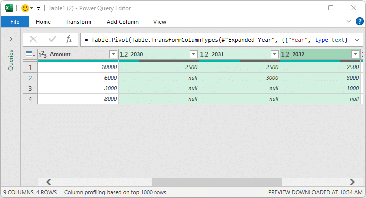
With our total amount now allocated into yearly columns, we can send the data back to an Excel worksheet. To do so, select Home and then Close & Load To … and select a Table in a new or existing worksheet as desired:

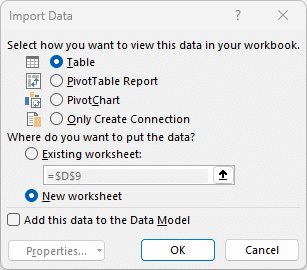
And Power Query creates the results table:

Optionally, you can add a total row to your table:

Select any cell in the results table, and go to Table Design and check the Total Row box.

You can add a Sum to any total row cell by selecting the cell and the choosing Sum from the drop down:

Now, the best part is that going forward, we don’t need to even open the Power Query editor to update our allocation for new contracts.

When you add new contracts to the source table, simply select Data and then Refresh All. Power Query will immediately update the results table to include any new (or changed) contracts.

Conclusion

And there you have it! By using Power Query, you can efficiently split amounts into annual columns and keep your data up-to-date with just a few clicks. If you have any questions or comments, feel free to leave them below.

Sample File

FAQs

Q: Can I use Power Query with older versions of Excel?
A: Power Query is available in Excel for Windows, 2013 and later versions.

Q: What if my source data has a total row?
A: You can apply a filter in Power Query to exclude the total row from the allocation.

Q: How do I handle errors in the custom column formula?
A: Ensure all references in the formula are correct and match your table’s column names.

Q: Is it possible to format the results table?
A: Yes, you can apply table styles and formats which will be retained upon refresh.