Format Items Found in a List

In this post, we’ll learn how to format a range to automatically highlight any items found in a list. In other words, we will learn how to highlight transactions that have a status value that matches any of the status values in a specific list, such as Pending or Processing. This illustration uses status values, however, the technique can be applied to highlight any transaction values that are equal to any values found in a separate list.

Video

Tutorial

To summarize our goal, let’s say we have a bunch of transaction like this:

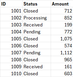
We want to highlight any transactions that have a status value found in our list:

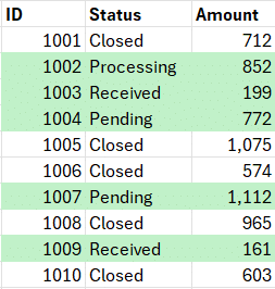
And when the conditional formatting rule is applied, the transactions with a Status value found in the Status Table is highlighted, like this:

Let’s cover the details of this type of Conditional Formatting with a few exercises.

Exercise 1: Understanding the MATCH Function

To kick things off, let’s familiarize ourselves with the MATCH function. This function is essential for finding the position of a value within a list. Here’s a quick example to warm us up.

Using the MATCH Function

The MATCH function looks for an item in a list and returns the position if found.

=MATCH(value, array, 0)

For example, let’s say we have a list of values in a Table named Table1:

This formula will return 1, which is the position of “Jan” within the list:

=MATCH("Jan", Table1, 0)

This formula will return 2:

=MATCH("Feb", Table1, 0)

And so on.

What if the value isn’t found? Since we used 0 for the third argument, the function returns an #N/A error if the value isn’t found in the range.

To recap, if the value is found in the range, a number is returned. If not, an #N/A error is returned.

But, when using formulas with Conditional Formatting, we’ll want the formula to return TRUE when the value is found in the range, and FALSE when it isn’t. So, let’s tackle that next.

Exercise 2: TRUE/FALSE

We would like to use a formula that returns TRUE or FALSE depending on whether the status is in the list. Currently, our MATCH function returns a number or an error. We can wrap the ISNUMBER function around it to have it return TRUE/FALSE instead, like this:

=ISNUMBER(MATCH(status, list, 0))

Note: if your version of Excel doesn’t support the ISNUMBER function, you can actually use the MATCH function alone in the conditional formatting rule in this case. For training purposes, I like to recommend formulas that return TRUE/FALSE whenever possible when using them as conditional formatting rules.

Now that we have a formula that returns TRUE when the status is found in the list, and FALSE when it isn’t, we can set up our Conditional Formatting rule.

Exercise 3: Conditional Formatting

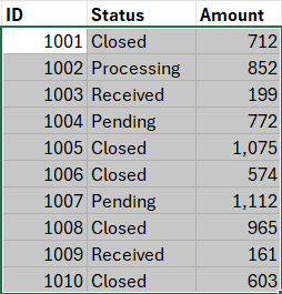
Now, let’s apply conditional formatting. First, select the range you’d like to highlight, like this:

Go to Conditional Formatting > New Rule > Use a formula to determine which cells to format.

Assuming the active cell within the selection is in row 14, the first Status cell in the data range is C14, and the status list is stored in cells B7:B9, enter the following formula (update references based on your worksheet as needed):

=ISNUMBER(MATCH($C14, $B$7:$B$9, 0))

Note:

• $C14 locks the column (C) but keeps the row (14) relative
• $B$7:$B$9 locks the row and column references to the status list
• 0 means exact match

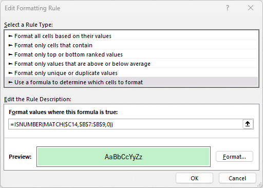
Pick your desired Format and click OK.

Now, conditional formatting highlights the rows where the status is found in our status list:

Mission accomplished!

Conclusion

And that’s how you can format items that appear in a list using Excel! I hope this tutorial was helpful. Feel free to leave comments or questions below. Thanks for joining me, and have a great day!

Sample File

FAQ

Q: What does the MATCH function do?
A: The MATCH function searches for a value in a range and returns its position.

Q: How do I lock cell references in a formula?
A: Use the dollar sign ($) before the column or row reference to lock it. For example, $C$14 locks both the column and row, while $C14 locks only the column.

Q: Can I apply conditional formatting to multiple columns?
A: Yes, you can select multiple columns and use a formula to determine the formatting criteria.

Q: Can I use other functions for conditional formatting?
A: Yes, Excel supports various functions for conditional formatting. The key is to write a formula that returns a TRUE/FALSE value. The other key is to use cell references based on the Active Cell. And the other key is to use absolute and relative references accordingly by assuming the formatting formula is filled throughout the selected range.

Q: What other formatting options can I use?
A: You can change font color, cell color, borders, and more through conditional formatting options.

Q: Is there a limit to how many statuses I can add?
A: Practically, there’s no limit. However, very large tables may affect performance.