Multi-Criteria Lookups with Copilot in Excel

Multi-criteria lookups are one of the most common challenges Excel users face. Whether we need to find a single matching record, retrieve a full list of matching rows, or sum up values across multiple conditions, the approach changes depending on the goal. In this tutorial, we walk through three exercises that show how Copilot in Excel can help us write the right formula for each scenario, using XLOOKUP, FILTER, and SUMIFS. Each exercise builds on the last, and by the end we will have a solid playbook for tackling multi-criteria lookups with confidence.

Exercise 1: Retrieve a Single Matching Record with XLOOKUP

Consider the following worksheet. We have a product table with columns for SKU, Product, Size, and Color. Above the table, we have a small lookup area where the user can enter a Product, Size, and Color. The goal is to write a formula in cell C10 that retrieves the matching SKU.

The tricky part here is that we have three conditions, not just one. A standard single-column lookup will not cut it. So, let’s get Copilot to help. We open the Copilot pane and type the following prompt:

Write a formula to retrieve the SKU based on selected product, size, color

Copilot reasons through the request and comes back with a formula. Before we look at what it generated, here is a quick introduction to the XLOOKUP function it chose to use.

In case we’re new to the XLOOKUP function, it searches a lookup array for a match and returns the corresponding value from a return array. The function arguments are:

• lookup_value: the value to search for
• lookup_array: the range or array to search
• return_array: the range or array from which to return a result
• if_not_found: value to return when no match is found (optional)
• match_mode: specifies the type of match, such as exact or approximate (optional)
• search_mode: specifies the search direction (optional)

Copilot generated the following formula and placed it directly into cell C10:

=XLOOKUP(1,(Table1[Product]=C7)*(Table1[Size]=C8)*(Table1[Color]=C9),Table1[SKU],"Not found")

This is a smart approach. Instead of looking up a text value, it looks up the number 1. The lookup array is constructed by multiplying three Boolean comparisons together. When all three conditions are true for a row, the math works out to 1, and XLOOKUP finds it. If none match, it returns “Not found”. We hit Enter, and bam:

With Hoodie, S, and Navy entered as criteria, the formula correctly returns SKU-201.

Mission accomplished for Exercise 1. But, what if multiple records could match our criteria? Well, let’s tackle that in the next exercise.

Exercise 2: Retrieve All Matching Records with FILTER

Now that we have handled the single-match scenario, it is time to deal with multiple matches. Let’s say we have a Transactions table with columns for Month, Vendor, Amount, and Category. The user can enter a Vendor and a Month, and we want to return ALL matching transactions, not just the first one.

XLOOKUP only returns the first match, so it is not the right tool here. We need something that can spill an entire filtered list. We open Copilot again and enter the following prompt:

Write a formula to retrieve Matching Transactions from the Transactions table that meet the Vendor/Month criteria

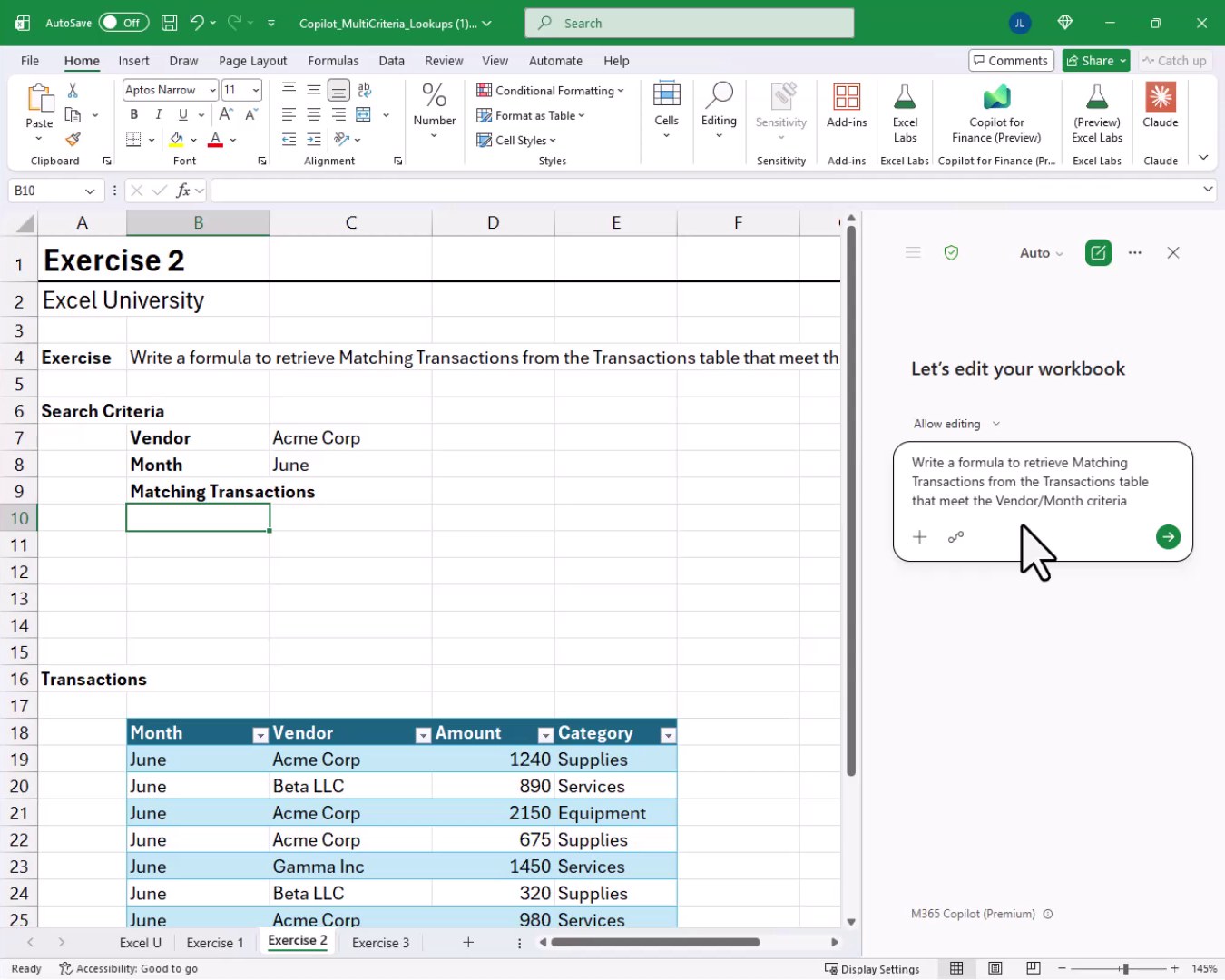
Copilot comes back quickly with a suggestion. Before we look at the formula, here is a quick look at the FILTER function it chose.

For those new to the FILTER function, it returns a subset of a range based on a condition, and the results spill into the surrounding cells automatically. The function arguments are:

• array: the range or table to filter
• include: a Boolean array the same height as array that determines which rows to return
• if_empty: value returned when no rows match the condition (optional)

Copilot generated the following formula and placed it in cell B10:

=FILTER(Table2,(Table2[Vendor]=C7)*(Table2[Month]=C8),"No matching transactions")

The same Boolean multiplication trick appears here. When both the Vendor and Month conditions are true, the row gets included in the results. If nothing matches, we see “No matching transactions” instead of an error. We fill the formula down, and bam:

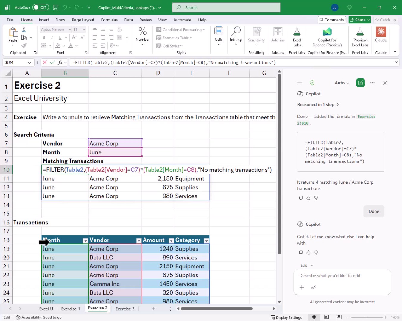
With Acme Corp and June entered as criteria, four matching transactions spill automatically into the worksheet.

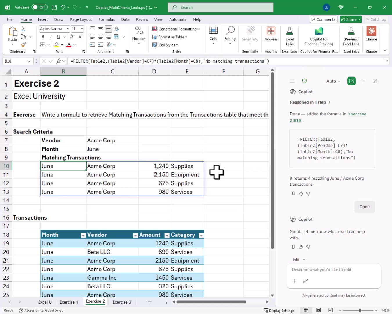
Change the vendor or the month and the results update instantly. That is FILTER doing exactly what it was designed to do. But, what if instead of listing all the rows, we just want a single total? Let’s bring this tutorial home.

Exercise 3: Sum All Matching Records with SUMIFS

Now, it is time to make things more interesting. In Exercise 3, we have a summary Report table with Rep and Region columns, and we need to fill in the Total Sales column. The source data lives in a separate Sales Data table with Rep, Region, Month, and Amount columns.

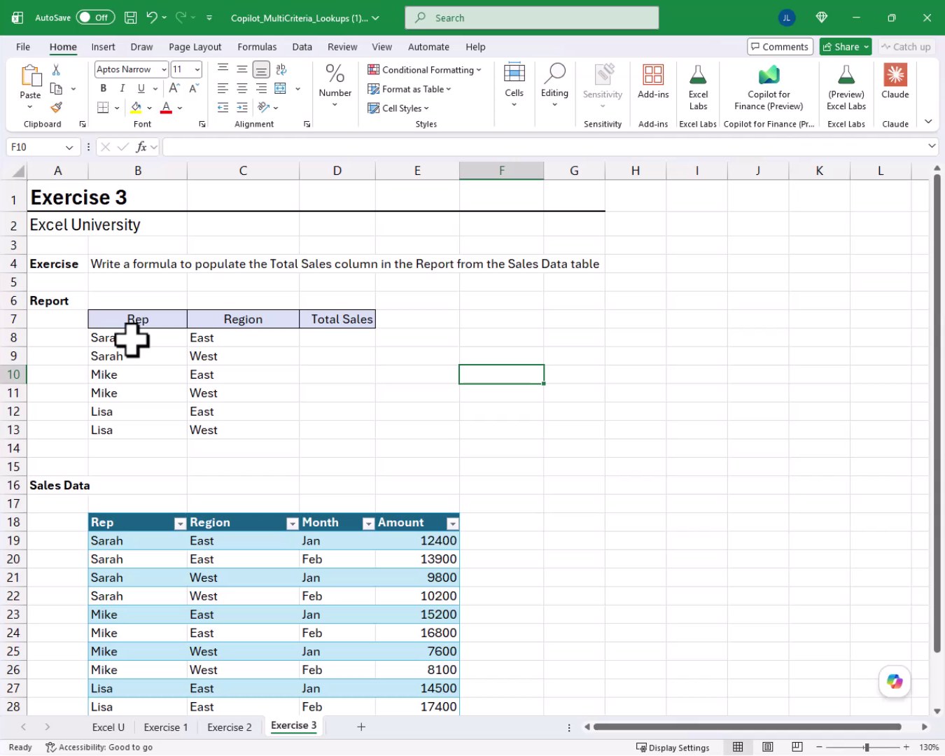
We need to sum the Amount column but only for rows where BOTH the Rep AND the Region match. We open Copilot and send it the following prompt:

Write a formula to populate the Total Sales column in the Report from the Sales Data table

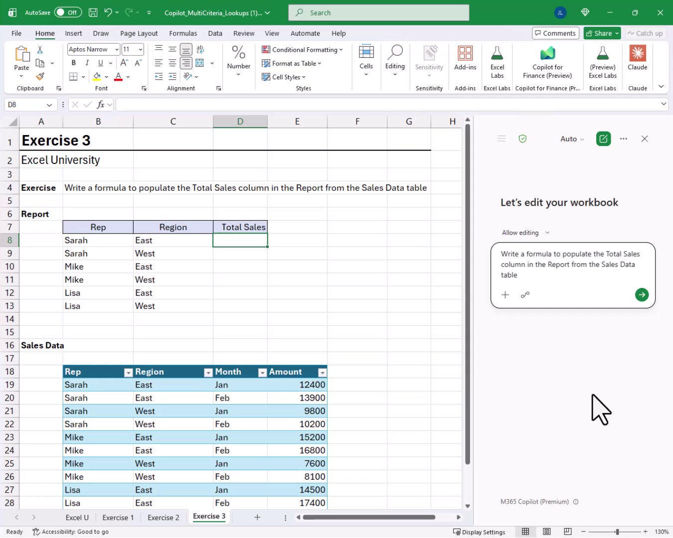
Copilot reasons through the structure of the workbook and picks exactly the right function. Here is a quick introduction to SUMIFS before we see the formula.

Before diving in, a quick look at the SUMIFS function. It returns the sum of values in a range that meet one or more conditions. The function arguments are:

• sum_range: the range of values to add up
• criteria_range1: the first range to evaluate against a condition
• criteria1: the condition that criteria_range1 must meet
• criteria_range2, criteria2, …: additional range and condition pairs, up to 127 pairs (optional)

Copilot placed the following formula into the Total Sales column, populating all six rows in a single step:

=SUMIFS(Table3[Amount],Table3[Rep],B8,Table3[Region],C8)

It sums the Amount column from Table3, but only includes rows where the Rep matches the Rep in our report row AND the Region matches the Region in our report row. Copilot even filled the formula into every row automatically, D8 through D13.

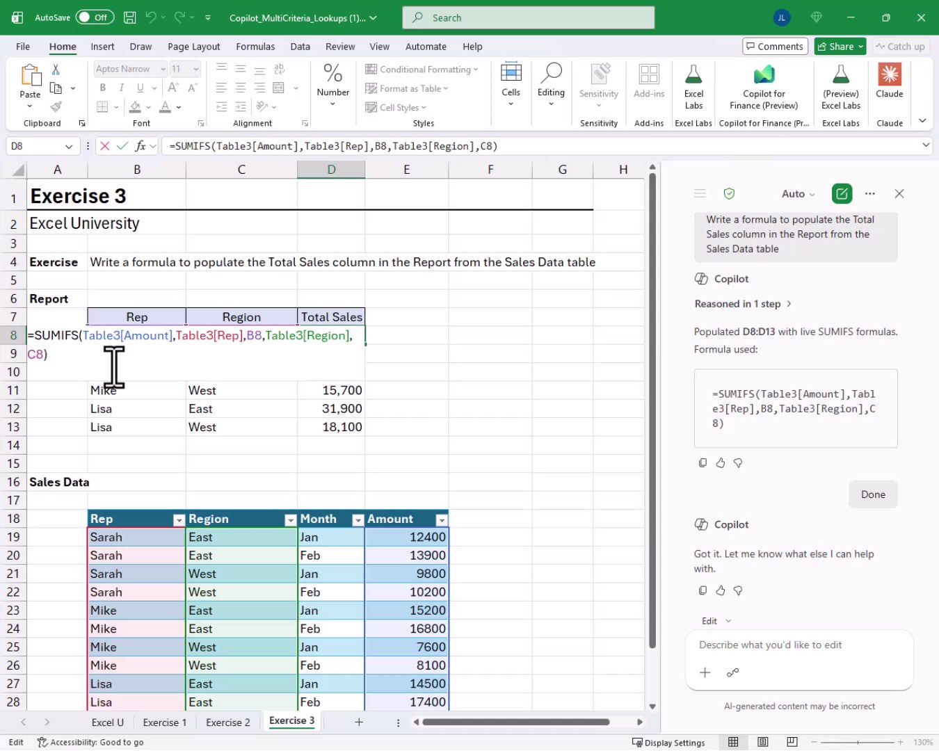
And when we inspect the completed report, bam:

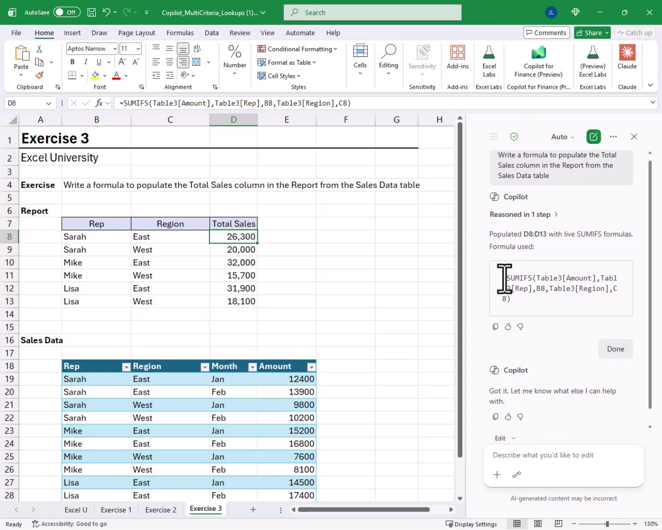
Every Rep and Region combination now shows the correct total. Sarah East shows 26,300. Mike West shows 15,700. Lisa East shows 31,900. All correct, all populated with a single Copilot prompt. And that is how we can use Copilot to write multi-criteria lookup formulas. Mission accomplished!

Summary

In this tutorial, we saw how Copilot in Excel can help us tackle three common multi-criteria lookup scenarios. When we need to return a single matching record, XLOOKUP with multiplied Boolean arrays gets the job done. When we need to return ALL matching rows, FILTER with the same Boolean multiplication technique spills the results automatically. And when we need the total of all matching records, SUMIFS handles it cleanly with multiple criteria range and criteria pairs. Copilot selected the right function for each scenario without us needing to specify it, which is a fantastic time saver.

If you have any suggestions, improvements, alternatives, or questions, please share by posting a comment below … thanks!

Sample File

FAQs

Does Copilot in Excel require a special subscription?

Yes. Copilot in Excel is part of the Microsoft 365 Copilot add-on, which requires a qualifying Microsoft 365 business subscription plus the Copilot license. It is not included in standard Microsoft 365 personal or family plans at this time.

Why does the XLOOKUP formula search for the number 1 instead of a text value?

When we multiply Boolean comparisons together, each comparison returns TRUE (1) or FALSE (0). A row where all three conditions are true evaluates to 1 times 1 times 1, which equals 1. XLOOKUP then searches for that 1 in the resulting array. It is a clever way to combine multiple conditions inside a function that normally only accepts a single lookup value.

Can we use XLOOKUP when multiple rows match the criteria?

XLOOKUP returns only the first matching row by default. If multiple rows could match, we should use FILTER instead, which is designed to return all matching records as a spilled array.

What happens if no records match the FILTER criteria?

By default, FILTER returns a #CALC! error when no rows match. That is why we use the optional third argument, if_empty, to return a friendly message like “No matching transactions” instead of an error.

Is FILTER available in all versions of Excel?

No. FILTER is a dynamic array function available in Excel 365 and Excel 2021 and newer. It is not available in Excel 2019 or earlier. Users on older versions would need to use array-based alternatives like INDEX/MATCH or consider upgrading.

Can SUMIFS handle more than two criteria?

Absolutely. SUMIFS supports up to 127 criteria range and criteria pairs. We can keep adding criteria_range and criteria arguments as needed to narrow the sum down to exactly the rows we want.

Can we write these formulas without Copilot?

Yes, and it is worth knowing how. XLOOKUP with Boolean multiplication, FILTER with multiplied conditions, and SUMIFS with multiple criteria pairs are all standard Excel techniques. Copilot just speeds up the process of getting there, especially when our data lives in named tables and the column references can get verbose.

Why does Copilot use structured table references like Table1[Product] instead of regular cell references?

When data is formatted as an Excel Table, structured references like Table1[Product] automatically expand as rows are added. Copilot recognizes the table structure and uses structured references accordingly, which makes the formulas more robust AND easier to read.

What if Copilot generates a formula that does not look right?

No worries, we can review the formula before accepting it. Copilot shows a preview of the formula in the pane before inserting it. We can also ask Copilot to explain the formula or request a revision by typing a follow-up prompt describing what needs to change.

Does Copilot always pick the best function for the job?

In most common scenarios, Copilot does a solid job selecting an appropriate function. However, AI-generated content can sometimes be incorrect, as Microsoft notes in the Copilot pane itself. It is always a good habit to verify the formula logic and test it against known results before relying on it in production.