Investment Evaluation Toolkit

When it comes to evaluating investments in Excel, most people immediately jump to the familiar NPV and IRR functions. While these are incredibly powerful, they can lead to incorrect conclusions if we don’t fully understand how they work, especially when cash flows vary or are irregular. In this post, we’ll walk through six powerful finance functions: PV, NPV, XNPV, IRR, XIRR, and MIRR. You’ll learn how to use them to make better informed investment decisions.

This post is brought to you by Finatical Software

• QuickBooks Online users! We know how essential Excel is for creating custom reports in the exact format you need. With Finatical, you can pull live, refreshable QBO financial data directly into your favorite Excel reports, no more copy, paste, export, repeat. It’s fast, easy, and built to streamline your workflow.
• A FREE TRIAL is available, so check it out risk-free today!

Video

Step-by-Step: Excel Investment Evaluation Functions

We’ll work through practical exercises to demonstrate how each of the following functions behave and when to use one over another:

• PV (Present Value) – Calculates the value today of future cash flows, factoring in a discount rate.
• FV (Future Value) – Determines how much a present investment will grow to over time at a given rate.
• NPV (Net Present Value) – Adds up the present value of a series of cash flows assuming equal time intervals.
• XNPV (Extended Net Present Value) – Similar to NPV, but allows for irregular timing between cash flows by using actual dates.
• IRR (Internal Rate of Return) – Finds the interest rate where NPV equals zero; shows the effective return of an investment.
• XIRR (Extended IRR) – Calculates IRR for cash flows that occur at irregular intervals using actual dates.
• MIRR (Modified IRR) – A more realistic IRR that factors in different rates for financing and reinvestment.

I’ll try to help you implement these functions into your workbooks and provide an understanding on timing assumptions, consistency in inputs, and related financial implications.

1. PV – Present Value

The PV function calculates what a series of future cash flows is worth in today’s dollars, adjusted by a given interest (or discount) rate. It lays the foundation for our time-value-of-money calculations. Excel’s syntax for this function is:

=PV(rate, nper, pmt, [fv], [type])

• rate – Interest rate per period
• nper – Total number of payment periods
• pmt – Amount paid each period
• fv – (Optional) Future value or a cash balance you want after the last payment
• type – (Optional) Payment type: 0 for end of period (default), 1 for beginning

Let’s put it to use with a example scenario.

Scenario: Compare two gym membership options: pay $1,000 upfront or $100/month for a year at a 5% annual interest rate compounded monthly. Well, these are difficult to compare since the timing is so different. $1,000 today vs $1,200 over time. One approach we can use to compare these, is to get the timing the same … in order words, compute the present value of each. The present value of $1,000 is easy … it is $1,000. But, how can we convert or translate the $1,200 paid over time all back into today’s dollars? Well, we can use Excel’s PV function to compute the present value. We set up the basic assumptions in our worksheet:

We need to make sure the function arguments use the same time period, for example, all annual or all monthly. Since our payment is monthly, we’ll need to ensure our rate is monthly (by diving by twelve), and the number of periods is monthly (by multiplying the number of years by twelve):

=PV(C13/12, C14*12, C12)

We hit Enter, and bam:

This tells us how much the $100 monthly payments are worth today. In our case, the result is $1,168. We can now compare that to the up-front option of $1,000 in order to make a more informed decision about our options.

Now that we are aware of present value with the PV function, let’s talk about net present value with the NPV function.

More on the PV function in this post.

2. NPV – Net Present Value

The NPV function calculates the present value of a series of future cash flows, allowing for varying amounts. It’s important to note that NPV assumes all cash flows occur at the end of each period.

Here’s the quick breakdown of the function’s arguments:

=PV(rate, nper, pmt)

• rate: the discount rate
• nper: the number of periods
• pmt: the payment per year

Let’s say we have a series of future cash flows with these basic assumptions (note the amounts are different for each year):

We can compute the net present value with the following formula:

=NPV(0.1, F11:F13)

To account for any initial investment (e.g., $500), we need to subtract it from the NPV results:

=NPV(0.1, F11:F13) - 500

Note: Don’t include the initial investment inside the values array of NPV unless it occurs at the future period start … Excel assumes all values in NPV happen at period 1 or later.

More on the NPV Function in this post.

3. XNPV – Irregular Cash Flow Dates

The XNPV function is essential when cash flows occur at irregular times, using actual date values instead of assuming regular periods.

XNPV Syntax:

=XNPV(rate, values, dates)

• rate: the discount rate applied to the cash flows
• values: the series of cash flows
• dates: the actual dates of the cash flows

This provides more precision and reflects actual cash flow timing, which can significantly impact investment evaluation.

For example, we can enter our cash flow amounts along with the actual dates, and compute net present value:

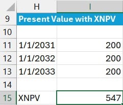
=XNPV(0.1, I11:I13, H11:H13)

More on the XNPV function in this post.

4. IRR – Internal Rate of Return

IRR finds the discount rate that sets NPV to zero, the break-even interest rate for an investment.

Syntax:

=IRR(values, [guess])

• values – An array of cash flows (must include at least one negative and one positive value).
• guess – Optional. A guess for what the IRR will be. Excel usually works fine without this.

It assumes regular timing of periodic cash flows. Use it to compare investment options and see which returns a higher yield. We enter our basic cash flow information into a range of cells and use the following formula to compute the internal rate of return.

=IRR(C8:C13)

More on the IRR function in this post.

5. XIRR – Internal Rate with Dates

XIRR improves on IRR by using real dates for each cash flow. This function returns the rate at which XNPV is zero.

Syntax:

=XIRR(values, dates, [guess])

• values: The array of cash flows, with the initial investment usually being negative.
• dates: The array of dates corresponding to each cash flow.
• guess: Optional. Our estimate for the IRR (Excel defaults to 0.1 or 10%).

We can enter the cash flows and dates into our worksheet, and then use the following formula to compute the internal rate of return.

This is a great choice when cash flows don’t occur annually or evenly as those timing differences can dramatically affect results.

More on the XIRR function in this post.

6. MIRR – Modified Internal Rate of Return

Both IRR and XIRR assume the positive cash flows are reinvested back into that project, and thus earn that same rate of return. But, if this assumption is not true, for example we pull cash flows out of the investment and put them into a savings account, we can use MIRR to specify custom finance and reinvestment rates. The basic syntax:

=MIRR(values, finance_rate, reinvest_rate)

• Finance rate: interest rate applied to negative cash flows
• Reinvestment rate: interest rate applied to positive cash flows

Example: You invest $10,000 and receive cash flows over five years. We enter the cash flows and dates, along with the assumed finance rate (applied to negative cash flow amounts) and reinvestment rate (applied to positive cash flow amounts) as follows:

=MIRR(C8:C13, C15, C16)

More on the MIRR function in this post.

Summary

Each function offers different strengths depending on your input structure:

• PV: Use for equal periodic payments.
• NPV: Use for uneven cash flows at regular intervals.
• XNPV: Use for uneven cash flows with actual dates.
• IRR: Find implied rate of return assuming regular intervals.
• XIRR: Use for irregular cash flow dates.
• MIRR: Use when you want realistic control over reinvestment and borrowing assumptions.

By mastering these functions and understanding their assumptions, we can confidently assess investment options, make data-backed decisions, and avoid costly misinterpretations.

Download the Practice Workbook

Ready to practice these Excel techniques? Download the sample file below and follow along with the examples:

FAQs

1. What is the difference between NPV and PV?
   

   PV assumes consistent payments over time, while NPV allows for varying cash flows.

   
   
2. When should I use XNPV over NPV?
   

   Use XNPV when cash flows occur at irregular intervals and you have specific dates.

   
   
3. Does IRR assume reinvestment of cash flows?
   

   Yes, IRR assumes all interim cash flows are reinvested at the same IRR rate.

   
   
4. How is MIRR different from IRR?
   

   MIRR allows for different financing and reinvestment rates, offering more realistic returns.

   
   
5. Can NPV and IRR give different investment recommendations?
   

   Yes. NPV shows absolute value created, while IRR shows percentage return. They can differ especially with non-standard cash flow timing or size.

   
   
6. What does a negative NPV mean?
   

   It typically indicates the investment won’t meet the desired rate of return or discount rate.

   
   
7. Why use XIRR for personal investments?
   

   Because it factors in the actual time value of money using real dates, making it perfect for personal irregular cash flows.

   
   
8. Should I include an initial investment in the NPV function?
   

   No, input it separately before or after the NPV for accurate calculations, unless it’s at period 1 instead of now (period 0).

   
   
9. What’s the default cash flow timing assumption in Excel?
   

   PV and NPV assume cash flows happen at the end of each period unless specified otherwise.

   
   

 Disclosures and Notes

• 100% of sponsor proceeds fund the Excel University scholarship and financial aid programs … thank you!
• This is a sponsored post for Finatical Software. All opinions are my own. Finatical Software is not affiliated with nor endorses any other products or services mentioned.