Inputs in Cells: How to Stop Hard-Coding Values in Excel Formulas

When we write Excel formulas, it is tempting to type a number directly into the formula. It works, sure. But the moment that number needs to change, we are stuck hunting down every formula across every worksheet. This tutorial shows a better approach: pulling those values out of our formulas, placing them in dedicated input cells, naming those cells, and then referencing the names in our formulas. The result is a workbook that is easy to update AND easy to maintain.

Exercise 1: The Problem with Hard-Coded Values

Let’s say we have a simple billing worksheet with work descriptions, quantities, and an Amount column we need to fill in. The amount is simply the number of hours multiplied by the hourly bill rate.

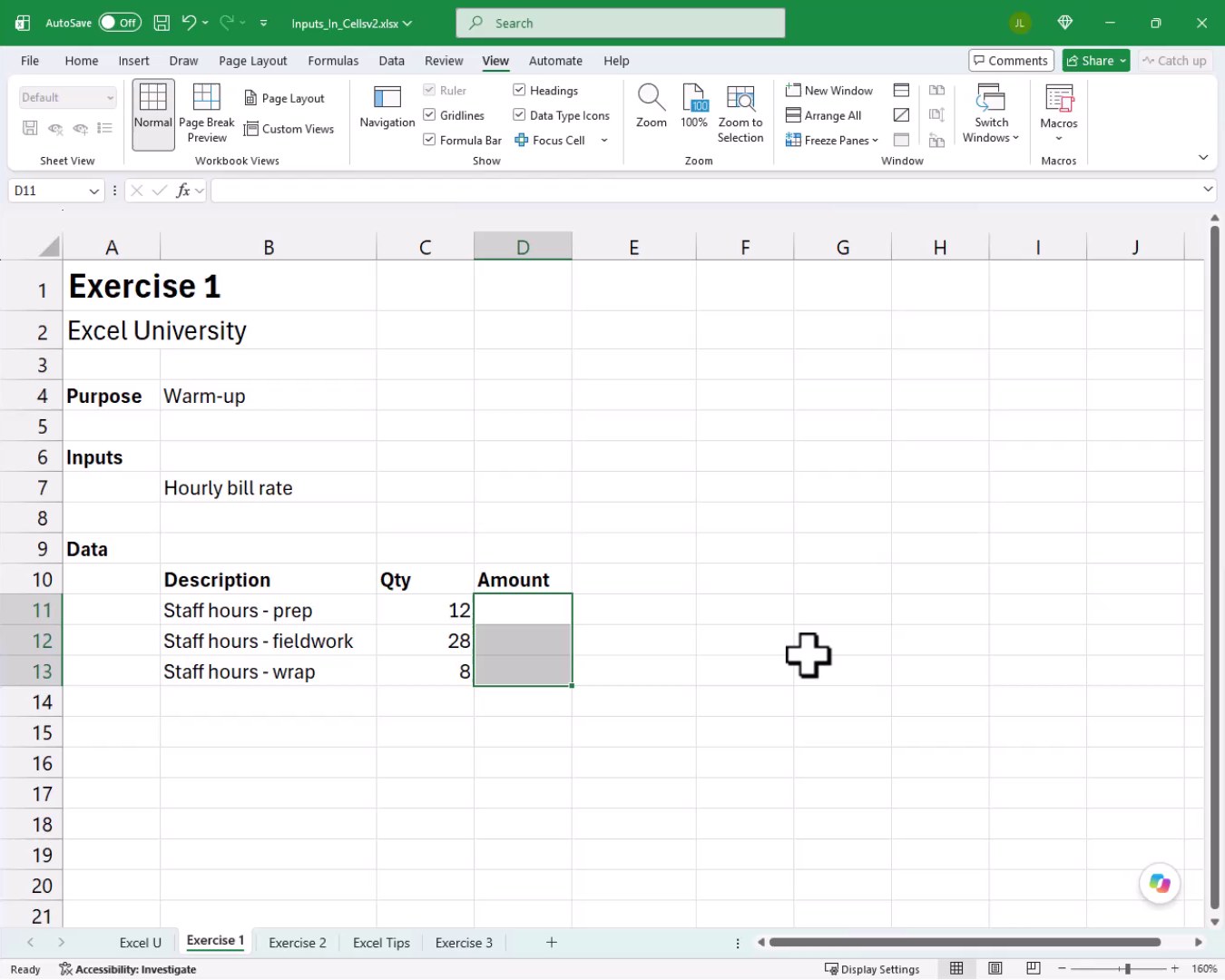
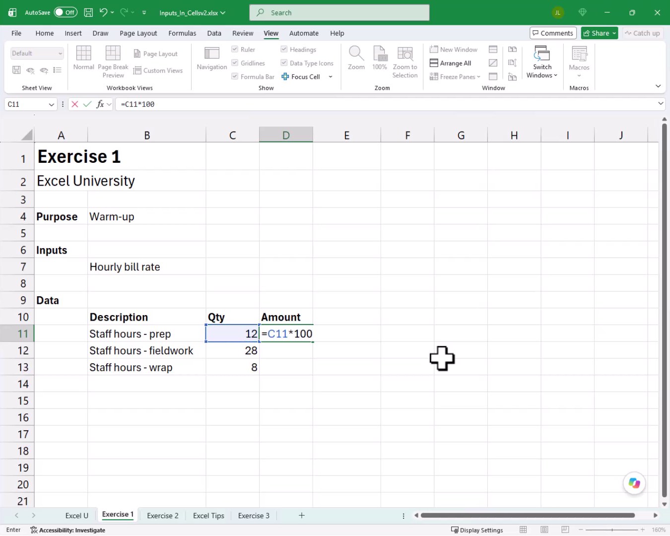
One option is to write the formula by embedding the rate directly into the formula, like this:

=C11*100

We fill the formula down, and bam, amounts appear for all three rows:

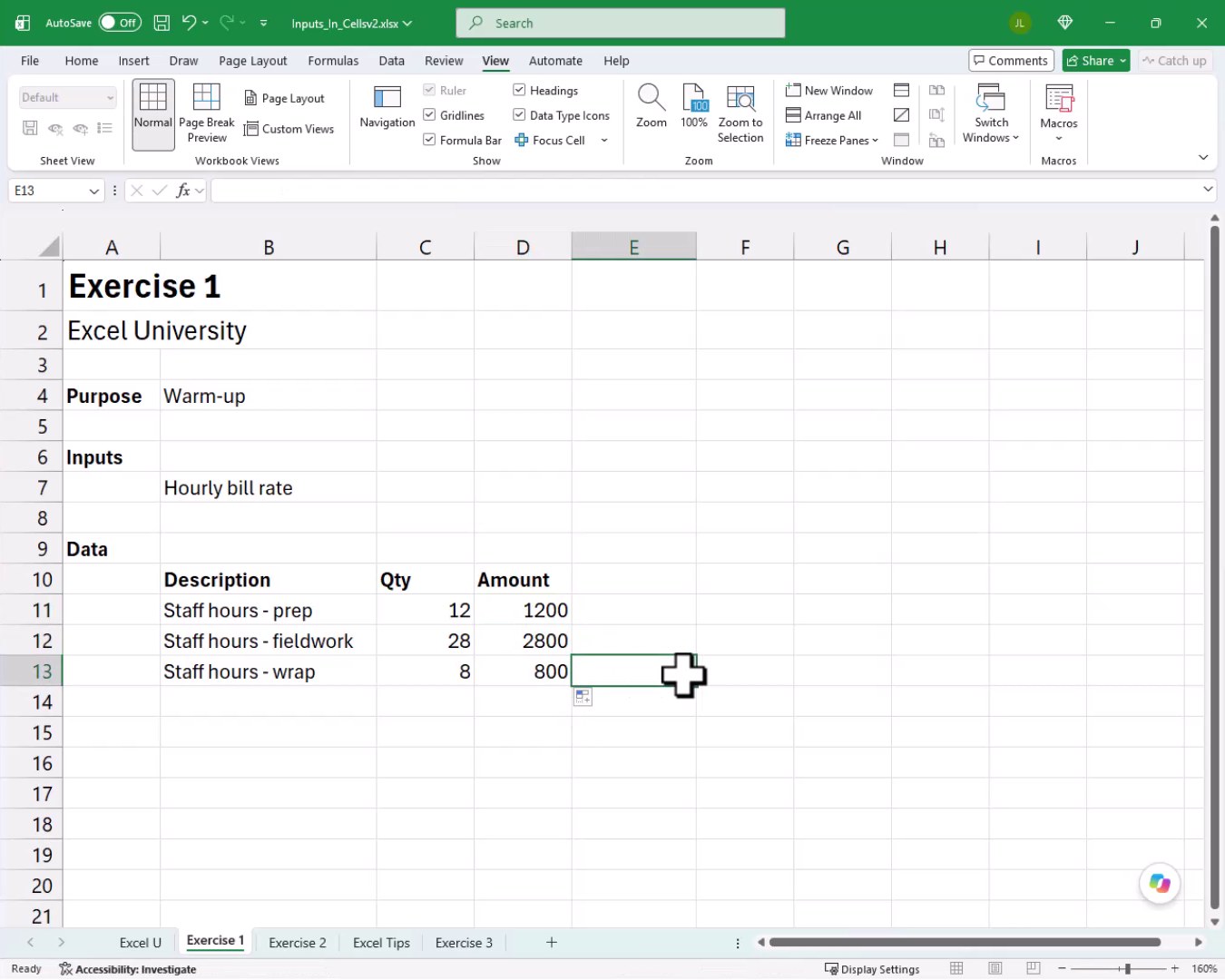
This works fine today. But next period, if the bill rate changes to 125, we have to hunt down every formula in every worksheet in this workbook that contains the hard-coded value 100. That is time-consuming and prone to errors. There is a much better way.

Exercise 2: Using a Named Range for the Input Cell

Now it is time to make things more interesting. Instead of hard-coding the rate, we place it in a dedicated cell. In Exercise 2, the hourly bill rate of 100 lives in cell C7. We want our formulas in the Amount column to reference that cell instead of the number itself.

Now, technically, we could solve this with an absolute cell reference using dollar signs. But there is an even easier approach: giving the cell a name. To do that, we click on cell C7 and then click inside the Name Box, which sits just to the left of the formula bar. We type the name we want to use.

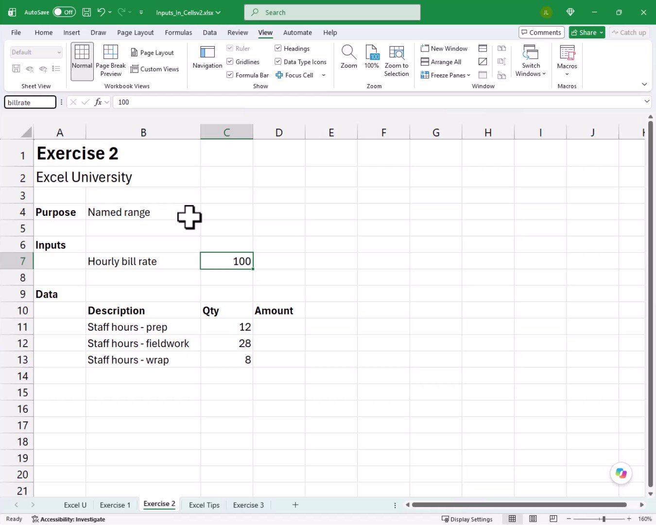
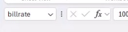
We type billrate into the Name Box and press Enter. It is important to press Enter after typing the name. If we just click another cell, the name will not be committed. Once we press Enter, the Name Box confirms our new name:

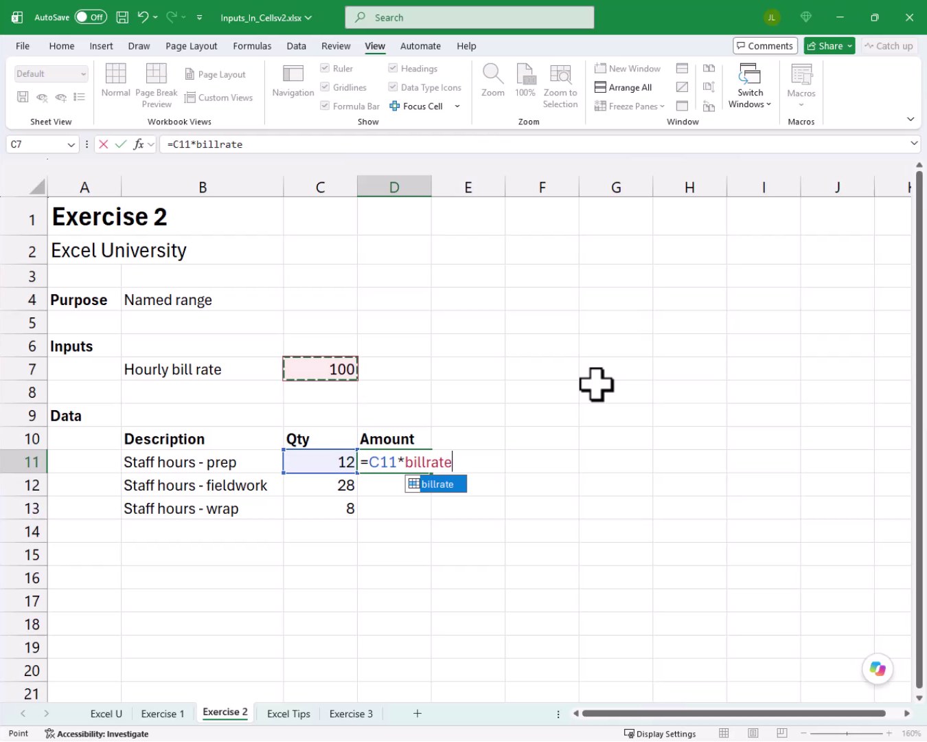
Now we write our formula in D11. As we type the multiplication symbol and then start selecting the input cell, Excel suggests the named range automatically:

=C11*billrate

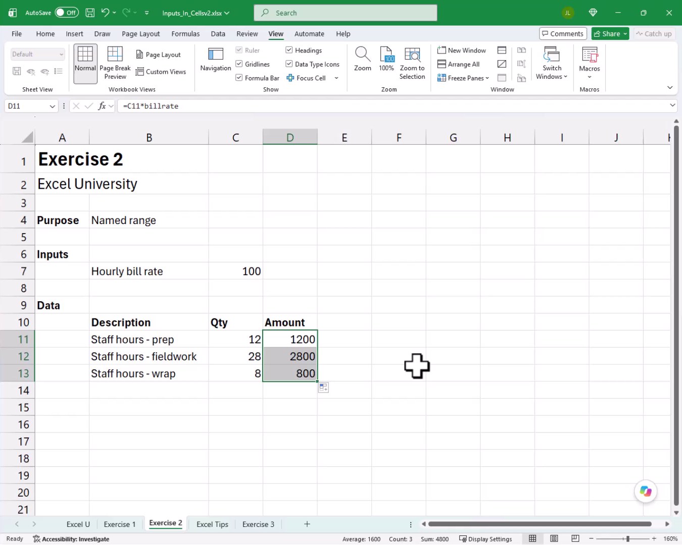
We hit Enter, and bam, the formula calculates correctly. We fill it down, and this time it works perfectly for all rows. Named ranges are absolute references by default, so no dollar signs are needed:

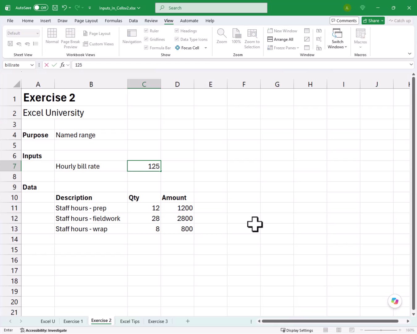
The real payoff comes when we need to update the rate. Instead of editing every formula, we simply type the new value into cell C7 and press Enter. Every formula referencing billrate recalculates instantly:

Exercise 3: Applying the Input Cell Style

With the named range approach in place, there is one more trick that makes our workbook even more user-friendly. When we share a workbook with colleagues, how will they know which cells to update and which cells contain formulas? Well … the answer is a cell style.

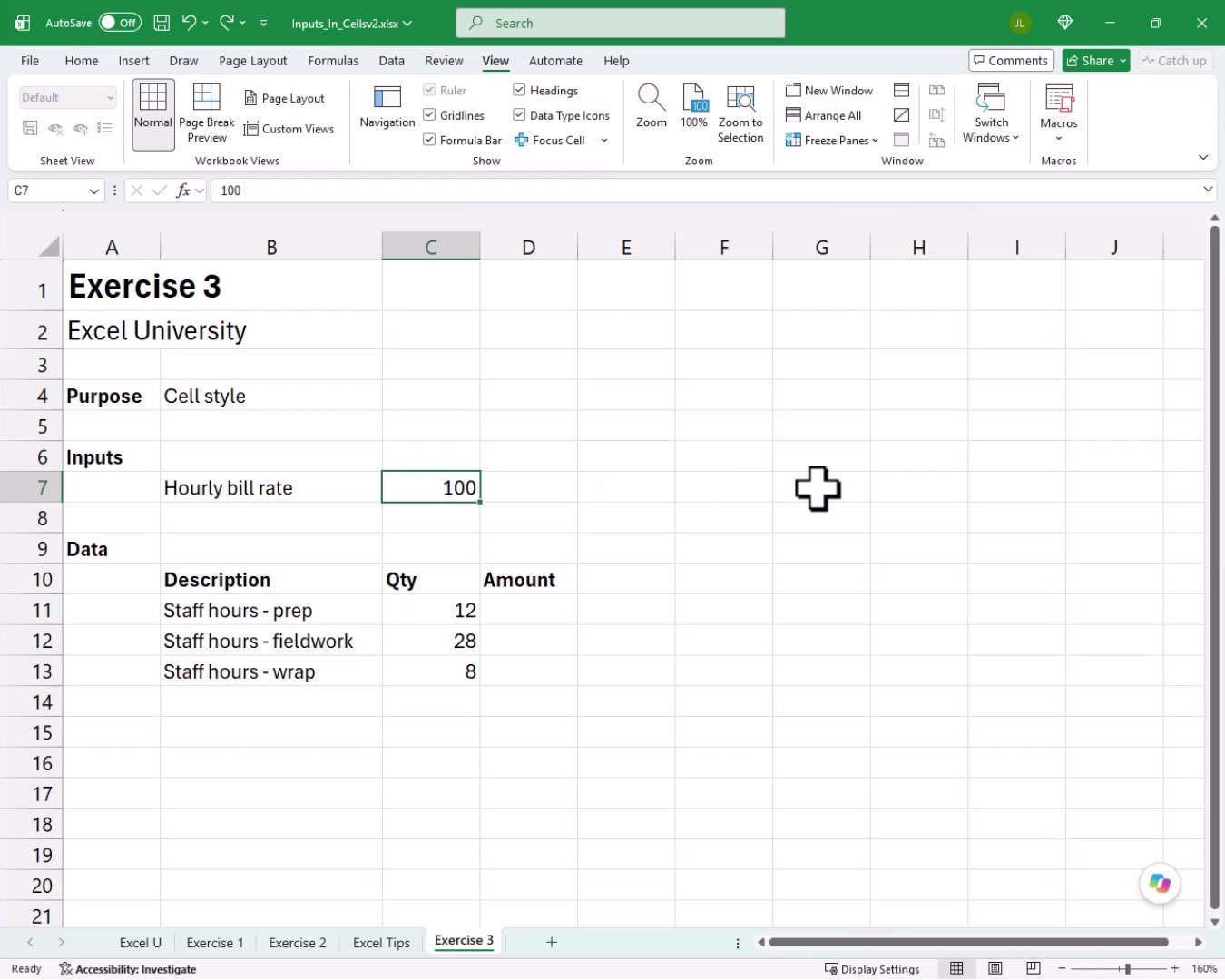
We select our input cell and give it a name using the Name Box, just as we did in Exercise 2. This time we call it hourlyrate. Then we write the same style of formula in the Amount column, referencing the named range. With the formula filled down and working, we move on to the cell style step.

On the Home tab, we click Cell Styles. Microsoft has actually included a style called Input specifically for this purpose. We can see it in the Data and Model section of the Cell Styles gallery:

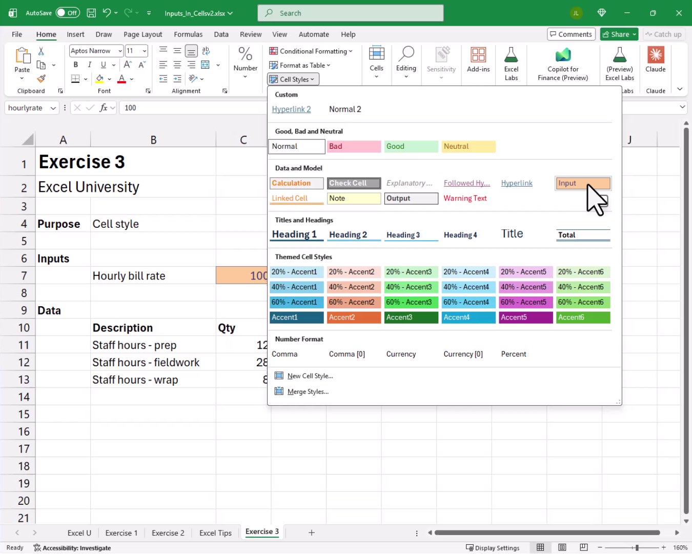
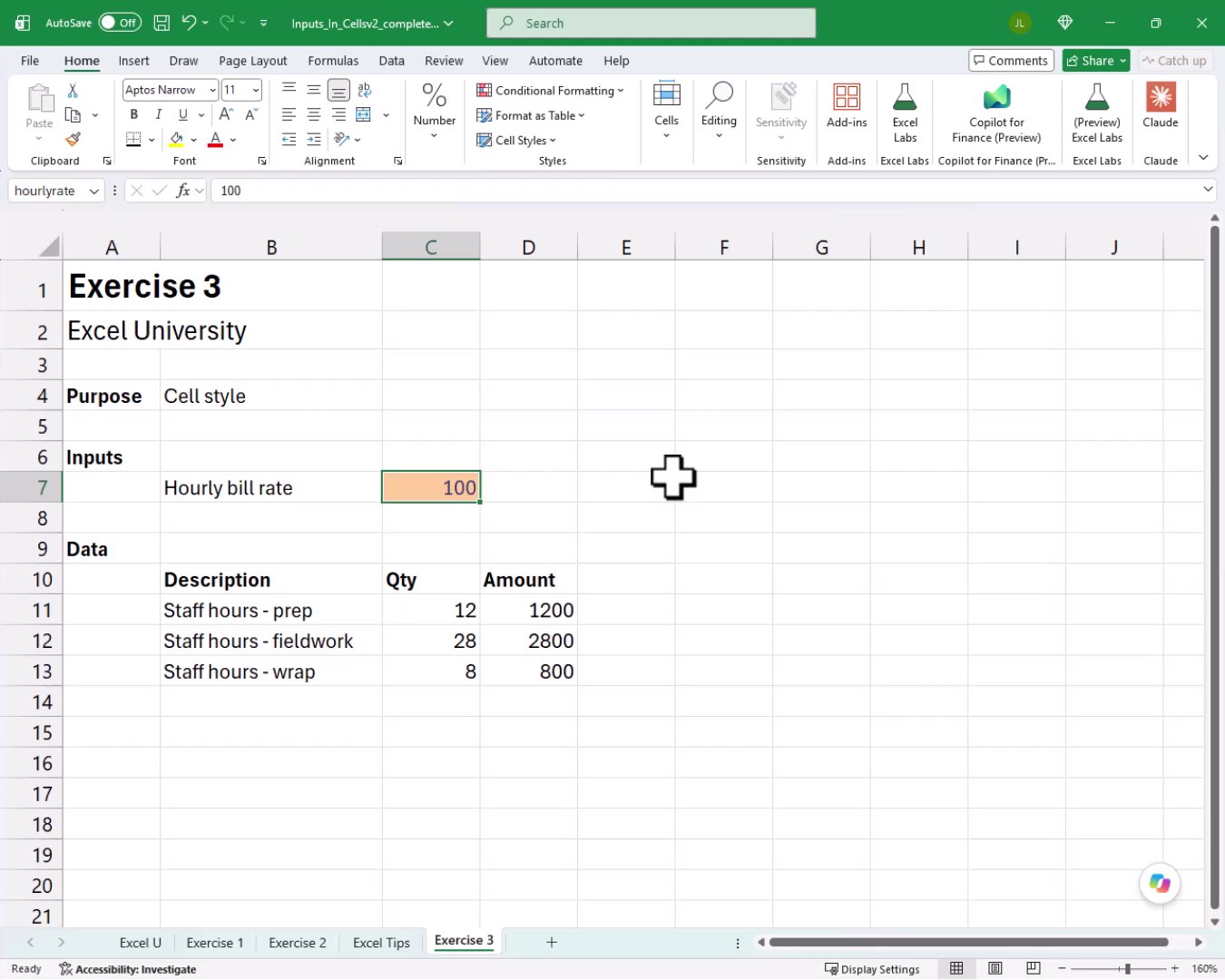
We click Input, and bam, the cell gets an orange background and orange text, making it immediately obvious to anyone opening the workbook that this is a cell that requires their attention:

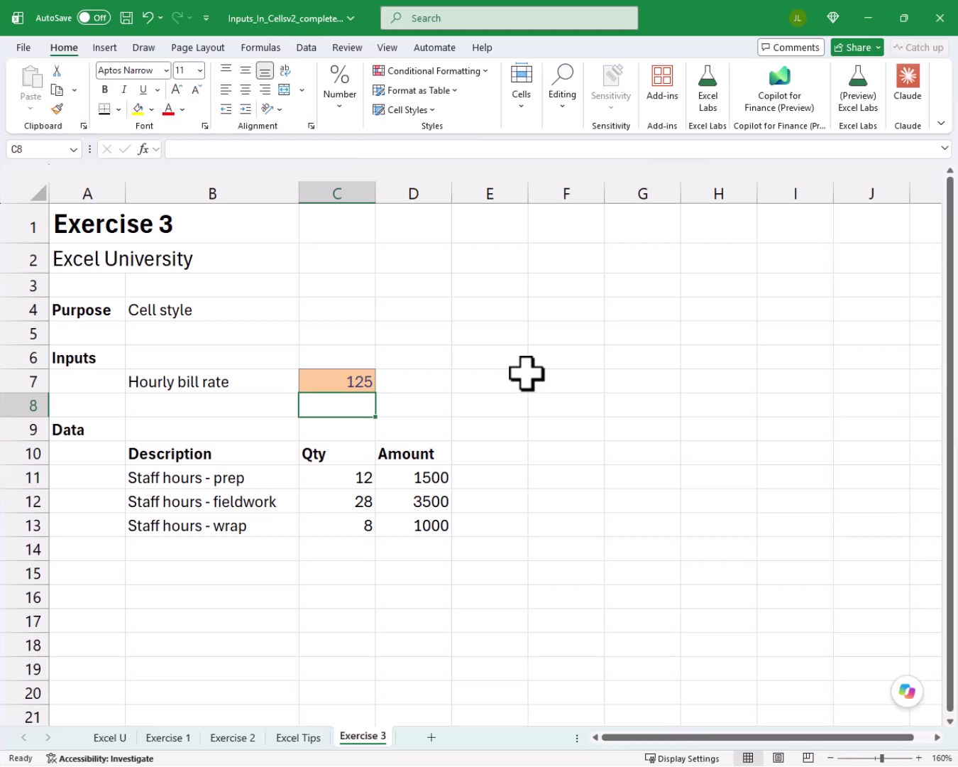
Now, when we need to update the rate, we update it in one place. We type 125, press Enter, and every formula in the workbook that references our named range updates automatically:

Summary

Rather than hard-coding values into our formulas, we can pull those values out into dedicated input cells. We give each input cell a descriptive name using the Name Box, reference that name in our formulas, and then apply the built-in Input cell style to make the input cells easy to spot. The result is a workbook that is easy to update, easy to share, and easy to maintain. Mission accomplished!

If you have any suggestions, improvements, alternatives, or questions, please share by posting a comment below … thanks!

Sample File

FAQs

What does it mean to hard-code a value in an Excel formula?

Hard-coding means embedding a number directly inside a formula, such as =C11*100. The number 100 is baked into the formula itself. If that number ever needs to change, we have to find and edit every formula that contains it, which is tedious and error-prone.

Why use a named range instead of an absolute cell reference?

Both approaches work. An absolute reference like =$C$7 locks the reference so it does not shift when filled down. A named range like billrate does the same thing automatically, without any dollar signs. Named ranges also make formulas much easier to read and understand at a glance.

How do we create a named range using the Name Box?

We select the cell we want to name, click inside the Name Box (the small box just to the left of the formula bar), type the desired name, and then press Enter. Pressing Enter is critical. If we click away instead, the name will not be saved.

Are there any rules for naming a range in Excel?

Yes. Named ranges cannot contain spaces or most special characters. A good practice is to use letters, numbers, and underscores only. The name also cannot start with a number or conflict with a cell address like C7. Descriptive names like billrate or hourlyrate work well.

What is the scope of a named range created through the Name Box?

By default, names created through the Name Box have workbook scope. That means the name is available on every sheet in the workbook, which is exactly what we want when formulas on multiple sheets need to reference the same input value.

How can we manage or delete named ranges?

We can manage all named ranges through the Name Manager. We get there by going to Formulas on the ribbon and then clicking Name Manager. From there we can create, edit, or delete any named range in the workbook.

What is the Input cell style and where do we find it?

The Input cell style is a built-in Excel style designed to visually identify cells that require user input. We find it by going to Home on the ribbon and clicking Cell Styles. It appears in the Data and Model section and applies an orange background with orange text by default.

Does this named range approach work across multiple worksheets?

Yes. Because the named range has workbook scope, formulas on any sheet can reference it by name. If the bill rate lives on a summary sheet and formulas on five other sheets reference billrate, updating the one input cell recalculates every formula across all five sheets instantly.

What happens to our formulas if we delete the named range?

If we delete a named range through the Name Manager, any formulas that reference that name will return a #NAME? error. To fix them, we either recreate the named range or update the formulas to reference a cell directly. It is a good idea to double-check formula dependencies before deleting any named range.