Formula-Based Reports with SUMIFS in Excel

Pivot tables are great, but they do not always produce the exact report layout that corporate requires. When the format is locked in and a pivot table simply will not fit, we turn to formulas. In this tutorial, we walk through three exercises that show how to use the SUMIFS function to build formula-based reports in Excel. We start with simple single-condition sums, move to cell-reference-based criteria, and finish by populating a fully formatted operating expense report with actuals, budget, variance, and variance percentage rows.

Exercise 1: SUMIFS with Static Values

Let’s say we have a transactions table with three columns: Department, Account, and Actual. Our goal is to sum the Actual column based on one or more conditions. Consider the following worksheet:

Before diving in, a quick look at the SUMIFS function. It returns the sum of values that meet one or more conditions. The function arguments are:

• sum_range: the range of values to add up
• criteria_range1: the first range to evaluate against a condition
• criteria1: the condition that criteria_range1 must meet
• criteria_range2, criteria2, …: additional range-condition pairs (optional)

Single Condition: Sales Department

We could write the following formula into cell E6 to sum all rows where the Department equals Sales:

=SUMIFS(tbl_Transactions1[Actual],tbl_Transactions1[Department],"Sales")

We hit Enter, and bam:

That is the total for the Sales department. One condition, clean and simple.

Two Conditions: Sales Department and Wages Account

We can extend the formula by adding a second criteria pair. To get the total where Department is Sales AND Account is Wages, we write:

=SUMIFS(tbl_Transactions1[Actual],tbl_Transactions1[Department],"Sales",tbl_Transactions1[Account],"Wages")

SUMIFS handles as many condition pairs as we need. Hardcoding text values in quotes works fine for a quick check. But, what if we wanted to make those criteria dynamic by pointing them at cells? Well, let’s tackle that in the next exercise.

Exercise 2: SUMIFS with Cell References and Mixed Addressing

Now that we have the basics down, it is time to make things more interesting. Exercise 2 introduces a small report grid with departments across the top (Corporate, Operations, Sales) and accounts down the left side (Wages, Salary, Overhead). We want a single formula in cell C7 that we can fill both down and to the right to complete the entire grid. Consider the following worksheet:

The key challenge here is getting the cell references right so the formula fills correctly in both directions. The department label sits in row 6 (C6, D6, E6) and the account label sits in column B (B7, B8, B9). As we fill across, we want the column to stay locked on B, but the row should move down. As we fill down, we want the row to be locked on 6, but the column should move right. That means we need mixed references.

So, we use the following formula in cell C7:

=SUMIFS(tbl_Budget[Budget],tbl_Budget[Department],C$6,tbl_Budget[Account],$B7)

With C$6, the dollar sign locks the row so it always points to row 6 as we fill down. With $B7, the dollar sign locks the column so it always points to column B as we fill across. We fill the formula down for the Corporate column, and bam:

Now, there is an important detail when filling this formula to the right. SUMIFS uses structured table references like tbl_Budget[Budget]. If we click and drag to fill right, Excel treats those column references as relative and rewrites them, which breaks the formula. Not a problem. We have two reliable options instead:

• Copy the formula (Ctrl+C) and paste (Ctrl+V) into the remaining columns. Excel treats structured table column references as absolute during a copy-paste.
• Select the formula cell and the empty cells to its right, then press Ctrl+R (Fill Right). This also preserves the structured table references.

We copy and paste across the remaining columns, and the grid fills in correctly:

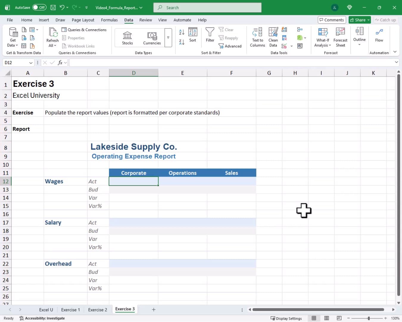
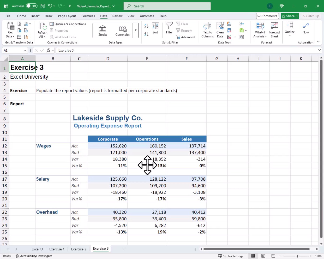
Exercise 3: Populating a Corporate Operating Expense Report

With the mixed-reference technique mastered, it is time to apply it to a real-world scenario. Exercise 3 presents a formatted operating expense report for Lakeside Supply Co. The report has accounts (Wages, Salary, Overhead) as row groups and departments (Corporate, Operations, Sales) as columns. Each account group has four rows: Act, Bud, Var, and Var%. Let’s take another look at our report template:

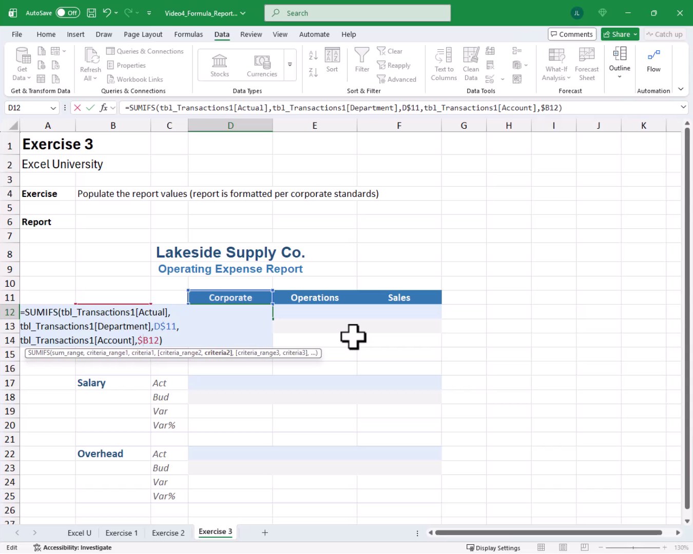
Pulling Actual Values

We start by writing the Actual formula in cell D12. The department headers are in row 11 and the account labels are in column B. We apply the same mixed-reference logic from Exercise 2. We write:

=SUMIFS(tbl_Transactions1[Actual],tbl_Transactions1[Department],D$11,tbl_Transactions1[Account],$B12)

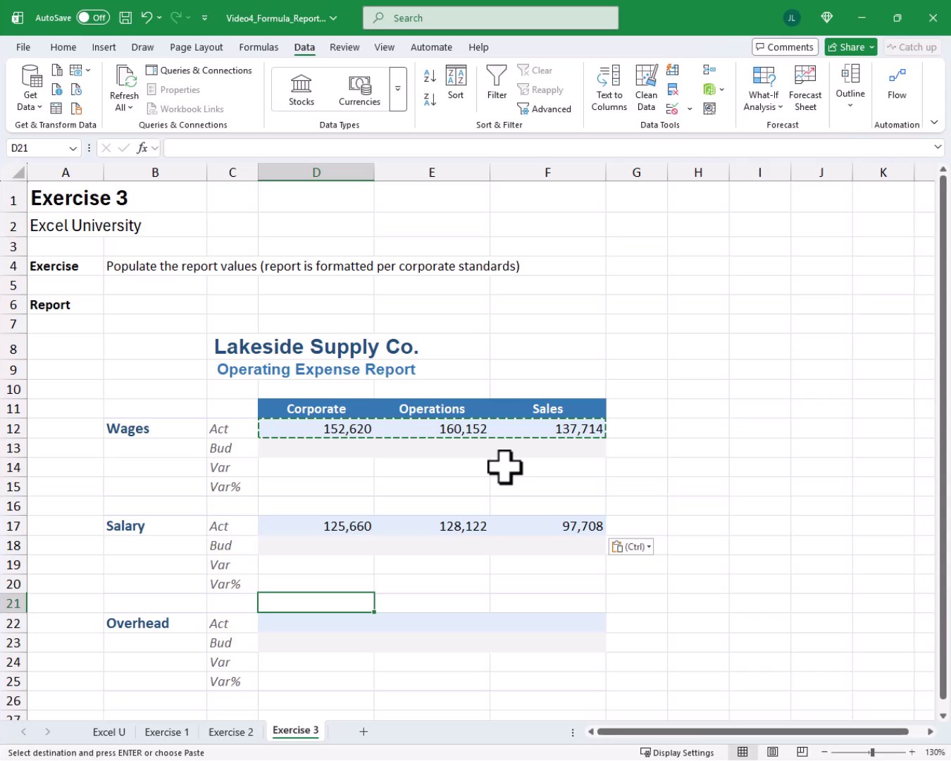
We hit Enter, confirm the result, then copy and paste the formula across the Operations and Sales columns. We fill the formula down, and bam:

Pulling Budget Values

The Budget rows follow the same pattern, but we point the formula at tbl_Budget instead. We write:

=SUMIFS(tbl_Budget[Budget],tbl_Budget[Department],D$11,tbl_Budget[Account],$B12)

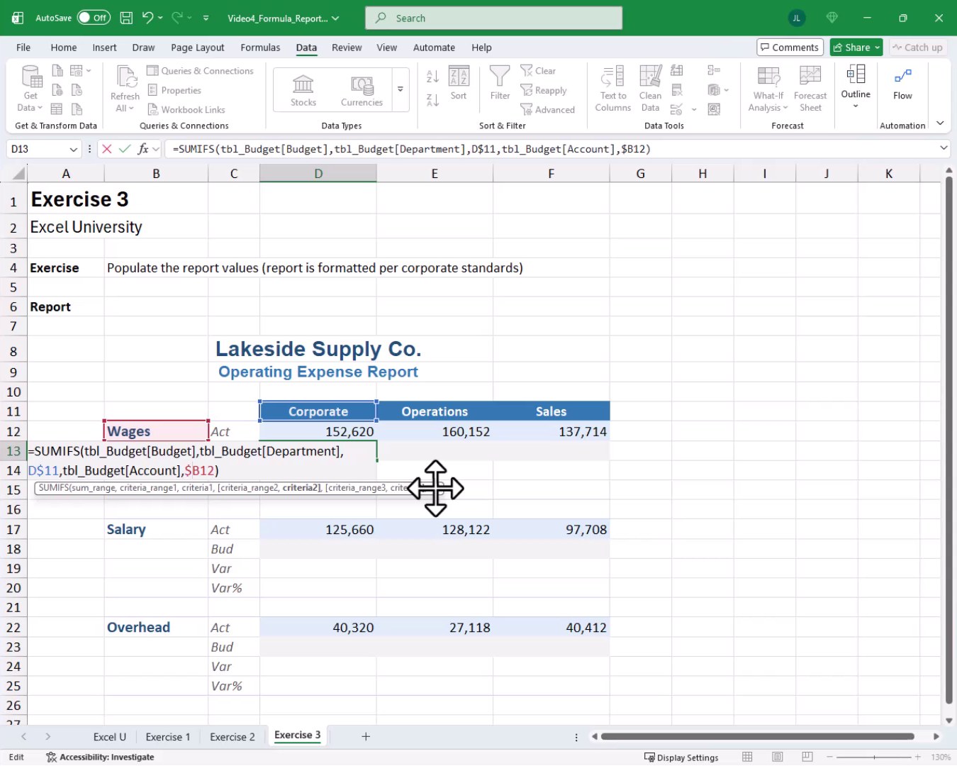
We copy and paste across all columns for each Budget row.

Variance and Variance Percentage

The Var rows are straightforward. Variance equals Budget minus Actual. We write that simple subtraction formula and fill right using Ctrl+R or copy-paste. The Var% row divides the variance amount by the budget amount. We copy and paste that across as well. The finished report looks like this:

Every cell is driven by a formula. When new rows are added to the transactions or budget tables, these formulas automatically pick them up. That is what makes this approach so powerful for recurring tasks like a month-end close. Mission accomplished!

Summary

In this tutorial, we used the SUMIFS function to build formula-based reports in three steps. First, we practiced SUMIFS with hardcoded static values using one and two conditions. Then, we replaced those static values with cell references and learned how mixed references (C$6 and $B7) let a single formula fill correctly both down and across. Finally, we applied everything to a real corporate operating expense report, pulling actuals and budget data from separate tables and computing variance rows. The result is a live, formula-driven report that updates automatically as source data grows.

If you have any suggestions, improvements, alternatives, or questions, please share by posting a comment below … thanks!

Sample File

FAQs

What is the difference between SUMIF and SUMIFS?

SUMIF supports only a single condition, and the argument order is criteria_range, criteria, sum_range. SUMIFS supports multiple conditions and puts sum_range first. Because SUMIFS is a superset of SUMIF and works with any number of criteria pairs, we prefer using SUMIFS in all cases for consistency.

Why do we use mixed references like C$6 and $B7 instead of fully absolute references?

A fully absolute reference like $C$6 would not move at all when we fill the formula, so every cell in the grid would look at the same header. Mixed references let us lock only one dimension. C$6 locks the row so the formula always reads the department header in row 6 regardless of how far we fill it down. $B7 locks the column so the formula always reads the account label in column B regardless of how far we fill it to the right.

Why does clicking and dragging to fill right break structured table references?

When we click and drag to fill right, Excel treats structured table column references as relative and rewrites them. So tbl_Budget[Budget] becomes tbl_Budget[Department], then tbl_Budget[Account], and so on, which is not what we want. Using copy-paste or Ctrl+R (Fill Right) instead tells Excel to keep those column references exactly as written.

Can we use SUMIFS with an Excel Table (structured references) and still fill the formula across?

Yes. The trick is to avoid click-and-drag fill when filling across columns. Using Ctrl+C followed by Ctrl+V, or selecting the range and pressing Ctrl+R, preserves the structured table column references so the formula works correctly in every column.

What happens when we add new rows to the source data table?

Because the SUMIFS formulas reference entire table columns like tbl_Transactions1[Actual] rather than fixed ranges like A1:A100, Excel automatically expands those references as new rows are added to the table. The report values update without any changes to the formulas. This makes formula-based reports ideal for recurring processes such as month-end reporting.

Can SUMIFS handle more than two conditions?

Absolutely. SUMIFS accepts up to 127 criteria range-criteria pairs. We simply keep adding comma-separated pairs after the sum_range argument. For example, we could add a third pair to filter by year, month, or any other column in the data table.

Is SUMIFS case-sensitive?

No. SUMIFS is not case-sensitive. A criteria value of “sales”, “Sales”, or “SALES” will all match the same rows. If case-sensitive matching is required, we would need a more advanced approach using array formulas or helper columns.

What versions of Excel support SUMIFS?

SUMIFS was introduced in Excel 2007, so it is available in essentially every modern version of Excel, including Excel 2007, 2010, 2013, 2016, 2019, 2021, and Microsoft 365. There are no version concerns with using this function in a shared workbook environment.

Can we use wildcard characters in SUMIFS criteria?

Yes. SUMIFS supports the asterisk (*) as a multi-character wildcard and the question mark (?) as a single-character wildcard when the criteria is a text value. For example, a criteria of “Corp*” would match Corporate, Corp, or any other text starting with Corp.

Why use a formula-based report instead of a PivotTable?

PivotTables are fast and flexible for exploratory analysis, but they have a fixed layout controlled by Excel. Formula-based reports let us design the exact layout, formatting, grouping, and row structure that corporate standards require. When the report template is locked in and must match a specific format every month, SUMIFS-powered formulas give us full control AND they update automatically as data grows.