Dynamic Pivot-style Report with GROUPBY

In this tutorial, we will learn how to use the GROUPBY function to create dynamic pivot-style reports with a single formula. Let’s back up a sec. For years, we’ve turned to PivotTables to build summary reports. Now we have another option: the GROUPBY function. While it doesn’t create a true PivotTable, it does create a similar report … a pivot-style report. And since it is built with a formula, it is totally dynamic … no need to click the Refresh command.

To demonstrate the GROUPBY function, I’ll walk through several exercises. Each will help to explain the various arguments and options available. By the end of this tutorial, you will be able to efficiently summarize and analyze your data using the GROUPBY function.

Video

Note: the GROUPBY function is NOT available in all Excel versions. At the time I’m writing this, it is being rolled out to Excel 365 users. Also, there is a similar function called PIVOTBY which supports column fields.

Step-by-step

Exercise 1: Creating a Basic Group By Report

The first exercise demonstrates how to create a simple summary report using the Account and Amount columns. This report will dynamically update when new accounts or data are added to the table.

Here is the data we’d like to summarize (Table1):

We can always use a PivotTable, and create something like this:

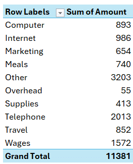
And that is how we’ve been summarizing data for years, and we still can. However, we now have a new option that is fully dynamic and automatically updates when the underlying data updates (no need to click Refresh).

The GROUPBY function has several arguments, for this exercise, we’ll look at only the first three arguments:

=GROUPBY(row_fields, values, function)

• row_fields is the data column that contains row items
• values is the column of values you’d like to summarize; typically a column of numbers
• function is the aggregate function to apply to the values field

Now, the function argument will feel a bit strange at first. This is because we enter a function name without parens and without arguments. This argument offers built-in lambda functions, technically knows as eta reduced lambda functions. Many are provided, and they include the ones you’d expect like SUM, MIN, MAX, AVERAGE, COUNT, and so on. If one of the functions listed in the drop-down isn’t sufficient, you can create your own LAMBDA function here.

To summarize Table1 by Account and show the sum of Amount, we would use the following:

=GROUPBY(Table1[Account],Table1[Amount],SUM)

We hit Enter, and bam:

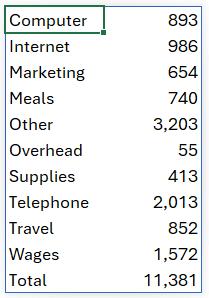
Wow! That is basically a pivot-style report created with a single formula! Since that formula returns multiple results (multiple cell values), Excel automatically spills the results into adjacent cells and will continue to use as many cells as needed as the underlying data in Table1 changes. So it’s fully dynamic!!

But wait, there more …

Exercise 2: Grouping by Multiple Row Fields

The second exercise demonstrates how to group by multiple row fields. Our source data (Table2) has AcctNum and Account name columns:

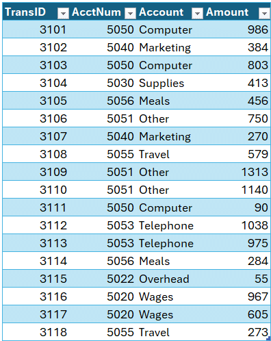
We’d like our report to show both account columns, and then sum the amount column. No worries, the GROUPBY function supports multiple row_field columns. We write the following formula:

=GROUPBY(Table2[[AcctNum]:[Account]], Table2[Amount], SUM)

And bam:

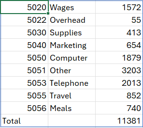
That entire report was generated by that single formula.

But, what if we want to display the columns in a different order than the data source? Or, what if they aren’t adjacent in the data source? Well, that’s where CHOOSECOLS comes in handy.

CHOOSECOLS

With CHOOSECOLS, you basically provide a full data range, like our table (Table2), and then identify by number the columns we want and in which order.

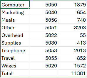
So, if we wanted the Account column (column 3) to be displayed before the AcctNum column (column 2), we use CHOOSECOLS as our first argument, like this:

=GROUPBY(CHOOSECOLS(Table2,3,2), Table2[Amount], SUM)

And bam:

But wait, there’s even more…

Exercise 3: Customizing Group By Reports

The third exercise illustrates the additional options available to customize the group by reports.

In addition to the first three required arguments, GROUPBY has four [optional] arguments. You’ll want to explore these based on what you are working on. Here is a quick summary:

=GROUPBY(row_fields, values, function, [field_headers], [total_depth], [sort_order], [filter_array])

• row_fields – column(s) to group by
• values – column(s) to summarize
• function – aggregate function used on values field
• [field_headers] – controls the display of column labels
• [total_depth] – grand totals, subtotals, above or below the data
• [sort_order] – which column(s) to sort by; negative to sort descending
• [filter_array] – expression to define which data rows to include

Let’s dig a little deeper into the function argument.

Function Argument

We have the standard aggregate functions you’d expect, like SUM, AVERAGE, and COUNT, but we also have ARRAYTOTEXT, which does this:

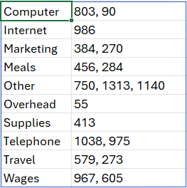
As you can see, instead of summing the values, it creates a comma-separated list of them.

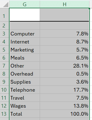
And we have PERCENTOF, which does this:

So, you’ll definitely want to explore the arguments so you can adapt them to your worksheet as desired.

Now, if you are like me, you’d really love to have some type of formatting applied to the total row. Maybe even just a cell border. But, since the report is dynamic, we know that the total row may move around to accommodate data changes. So, if we don’t want to have to manually format and reformat with each data change, what can we do?

Well, good news … we can do that with conditional formatting. That way, as the dimensions of the report change (since it is dynamic), conditional formatting with keep up with the changes and apply the formatting automatically.

Applying Conditional Formatting

To add conditional formatting, follow these steps:

Select the columns where you want to apply conditional formatting, for example, G:H.

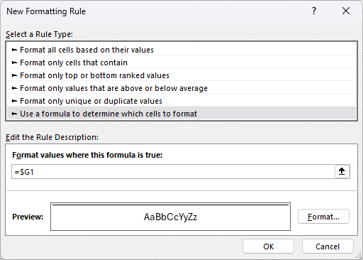
Next, Home> Conditional Formatting > New Rule > Use formula to determine which cells to format.

In the resulting dialog, write a formula that points to the first cell in the column that contains the word “Total” in the report (which is also the active cell). Be sure to use an absolute column relative row reference, such as $G1. Then Format and choose a top cell border.

Now the top cell border will be applied to the Total row, like this:

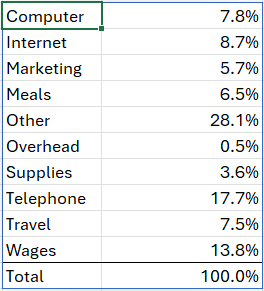
And the good news is that the formatting will dynamically adjust as new rows or accounts are added to the report.

Conclusion

Excel’s GROUPBY function provides a powerful and dynamic way of creating pivot-style reports without the need for multiple formulas or a formal PivotTable. So, for simple reports, this provides a great alternative. Now, PivotTables are still the way to go for fully interactive reports that include all of the robust PT capabilities.

If you have any suggestions, alternatives, or questions … please share by posting a comment below, thanks!

Sample File

FAQ

Q: Can I use the GROUPBY function in older versions of Excel?

A: The GROUPBY function is rolling out to Excel 365 users, and will not be retro-fit back into older versions of Excel.

Q: Does the GROUPBY function automatically update when new data is added to the table?

A: Yes, the GROUPBY function is dynamic. It will automatically update when new data is added to the table without the need for manual refreshing.

Q: Can I group by non-adjacent columns in the table?

A: Yes, by using the CHOOSECOLS function as the first argument of the GROUPBY function. See Exercise 2 above for details.

Q: Can I apply conditional formatting to the report?

A: Yes, you can apply conditional formatting to the report. An example of this is provided in Exercise 3 above.