How to Find Invalid Characters

Welcome to this tutorial on how to find invalid characters in Microsoft Excel. In this tutorial, we will explore different methods including formulas and conditional formatting to detect and highlight characters you define as “invalid” in your Excel worksheets. Since you can easily customize the list of “invalid” characters, this approach is extremely flexible and can be used in many different situations.

Video

Step-by-step

To illustrate the steps, I’ve created three exercises. You can grab the file using the link below if you’d like.

Exercise 1: Using the FIND Function to Find Invalid Characters

We begin by defining a list of invalid characters and storing them in a table. For illustration purposes, I’ll keep the list short. The table is named Table1:

Note: if you haven’t created a Table before, head to Insert > Table. You can name the table if you wish by using the Table Name field, otherwise, the default name is Table1.

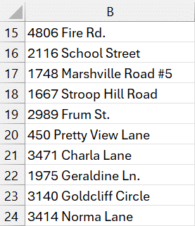
Now, we have a bunch of cells, and we want to see if any of them contain any of the characters in Table1.

One option is to write a formula in an adjacent column that uses the FIND function. For example, in cell C15, we can use the following formula:

=FIND(Table1, B15)

This formula looks for the characters in Table1 in the cell B15.

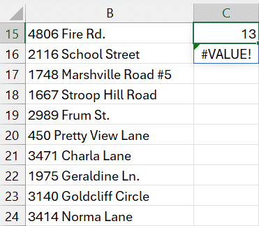
You’ll notice that our single formula returns two results … one for each character in Table1. If the FIND function returns a number, it means the character is found at that position number. If FIND returns an error, the character is not found.

Note: FIND is case sensitive and doesn’t support wildcards. Depending on what you are working on, you may consider using SEARCH instead which is case insensitive and supports wildcards.

So, in this example, the table has two characters so two results are returned. The first result is 13, which means that the first “invalid” character was found at position 13 in B15. The second result is the #VALUE! error, which means the second character in the list was not found.

But, we need a way to sort of collapse all of these results into a single cell. One option would be to use the COUNT function. It will count the number of cells with a value and ignore errors. So, we can update our formula as follows:

=COUNT(FIND(Table1,B15))

We hit Enter, and bam:

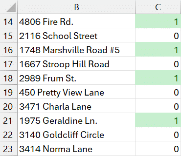
We can fill this updated formula down to apply it to the remaining cells in our helper column:

If the result is 0, none of the “invalid” characters (as defined) are found. If the results are >0, then an invalid character has been found.

Bonus

If you’d like to convert the results column to checkboxes using the Checkbox Cell Control (as discussed in my previous post) you can convert the formula results to Boolean values by use a comparison operator as follows:

=COUNT(FIND(Table1,B15))>0

This returns TRUE/FALSE instead of the count. You can then select the formula range and use the Insert > Cell Controls > Checkbox command and bam:

Note: the Insert > Cell Controls > Checkbox command is NOT available in all Excel versions. At the time of this writing it is being rolled out to Excel 365 users.

Note: if you want to check the boxes that do not have the invalid characters, update the formula to: COUNT(FIND(Table1,B15))=0

Exercise 2: Applying Conditional Formatting

Let’s say we’d like to apply conditional formatting to highlight the cells that contain any invalid characters.

Well, one straightforward option would be to conditionally format the helper column. We start by selecting all of the formula cells in the helper column.

Next, we go to Home > Conditional Formatting > Highlight Cell Rules > Greater Than. In the resulting dialog we set the condition to 0 and pick the desired formatting.

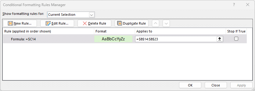
Instead of formatting the helper column C, we could format data column B. Begin by selecting the range and then Home > Conditional Formatting > New Rule > Use a formula to determine which cells to format. In the resulting dialog, we set the formula equal to the first helper column cell using an absolute column relative row reference:

Click OK to apply the conditional formatting:

But, what if we wanted to remove the helper column? Well … that leads us to our final exercise.

Exercise 3: Removing the Helper Column

In this exercise, we’ll effectively move the logic of the helper column formula into the conditional formatting rule. That way, we eliminate the need to display the helper column in the workbook.

First, we’ll define a name for the table reference using the Name Manager. Formulas > Name Manager > New. Give it a name (like “chars”), and in the “Refers to” field, enter the name of the table.

Click OK to create the defined name.

Select the cells you want to apply conditional formatting to, and Home > Conditional Formatting> New Rule > Use a formula to determine which cells to format.

In the formula field, enter:

=COUNT(FIND(chars, B14))

Select a format and click OK to apply the conditional formatting.

As you can see, we essentially moved our helper formula into the conditional formatting rule, thus eliminating the need to display it in the worksehet 🙂

Conclusion

Congratulations! You have learned how to find invalid characters in Excel using formulas and conditional formatting. By following the steps in this tutorial, you can easily identify and address any invalid characters in your data. Start exploring and utilizing these techniques to ensure the accuracy and integrity of your Excel worksheets.

If you have any alternatives, suggestions, or questions, please share by posting a comment below … thanks!

Sample File

FAQ:

Q: What is an invalid character in Excel?

A: For the purposes of this post, we define a set of characters that we want to find. They aren’t invalid in the sense that Excel doesn’t allow them. They are invalid because we defined them as such, and the approach presented in this post makes it very easy to customize the list of “invalid” characters as desired.

Q: Can I find invalid characters in a specific column only?

A: Yes, you can apply the FIND function and conditional formatting to a specific column by selecting the range of cells and adjusting the formulas accordingly.

Q: How can I remove the conditional formatting if no longer needed?

A: To remove conditional formatting, select the formatted cells, go to the Home tab, click on Conditional Formatting, and choose “Clear Rules”.

Q: Can I use wildcards to find invalid characters?

A: Yes, you can use the SEARCH function, which supports wildcard characters, instead of the FIND function which does not. Please note that the FIND function is case sensitive and the SEARCH function is not.