Dynamic Date Report Header For The Period Ending

As a general rule, it is a good idea to delegate as many tasks to Excel as possible. Report headers are no exception, especially for recurring-use workbooks. This post explores the functions needed to create a dynamic report header, such as “For the Period Ending December 31, 2015.”

Overview

Let’s assume we use the same workbook each year to prepare a report. Most likely, the report includes a header that tells the reader the effective date of the report. For example, a profit and loss statement may indicate “For the Periods Ending December 31, 2015 and 2014.” Or, a balance sheet may use “As Of December 31, 2015.” The goal is to have Excel automatically update all of the date headers throughout the workbook once we enter the effective date into a single cell. Fortunately, there are only a few worksheet functions needed to accomplish this.

Functions

Let’s begin by showing a screenshot of our Start Here sheet, where we enter the effective date used throughout the workbook:

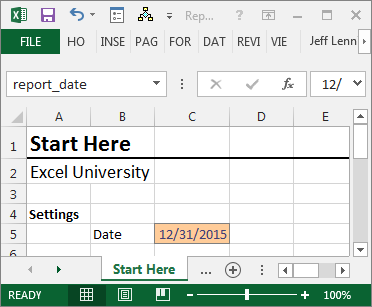
For convenience, I’ve named the date input cell report_date, as seen in the Name Box above.

When we enter a new date, we would like all of the report headers to update accordingly. The first function we’ll need is the CONCATENATE function.

CONCATENATE

The CONCATENATE function allows us to join values. It returns a text string that combines all of its arguments. For example, the following formula would return the text string “Excel University”

=CONCATENATE("Excel", " ", "University")

In addition to the CONCATENATE function, you can use the concatenation operator the ampersand &. It is just personal preference which to use, they both achieve the same result. The following formula would return the text string “Excel University”:

="Excel" & " " & "University"

Before we convert the static report header into a formula, let’s see what the worksheet looks like:

To have Excel provide the report header, we start by writing the following formula:

=CONCATENATE("For the Period Ending ",report_date)

Where:

• “For the Period Ending “ is the first argument, and includes a trailing space
• report_date is the name of the cell that stores our report date

At this point, when we hit enter, we get the following worksheet:

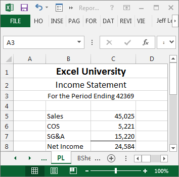
Wait, what! Our formula returns “For the Period Ending 42369” which is certainly not what we wanted. This is because the CONCATENATE function, like other Excel functions, operates on the stored value, not the displayed value. That means any date formatting applied to the input cell is disregarded. In order to format the date serial number 42369 as a date, we’ll need to enlist the help of the TEXT function.

TEXT

The TEXT function returns a text string with a specified format. The syntax follows:

=TEXT(value, format_text)

Where:

• value is the value to format
• format_text is the format definition to apply, surrounded by quotes

Since the format_text argument supports the standard custom format codes, such as mmmm for the full month name, d for the day, and yyyy for the four-digit year, we can wrap a TEXT function around the report_date argument as follows:

=CONCATENATE("For the Period Ending ",TEXT(report_date,"mmmm d, yyyy"))

Ah yes, much better! Here is the updated report:

And, what if we had comparative statements? No problem, for that, we’ll need to enlist the help of the YEAR function.

YEAR

Let’s take a quick look at the report:

The YEAR function returns the year of the date argument. So, we can figure out the year of the report_date cell as needed for cell C5 by using the following formula:

=YEAR(report_date)

And, we can use the following formula to figure out the prior year as needed for cell D5:

=YEAR(report_date)-1

And finally, we can update the report header formula as follows:

=CONCATENATE("For the Periods Ending ",
TEXT(report_date,"mmmm d, yyyy"),
" and ",
YEAR(report_date)-1)

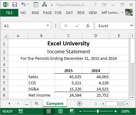
The best part is that when we update the date input cell, all of the report headers update accordingly, as illustrated below:

Bam!

Conclusion

To really make this report awesome, we would want to use the SUMIFS function to compute the report values based on the source data table. If you’ve not yet explored the SUMIFS function, please check out the blog post referenced below. If you have any other approaches or ideas, please share them by posting a comment below…thanks!

Additional Resources

• Sample file download: ReportHeaders
• SUMIFS blog post: SUMIFS