Currency Exchange Rates

Manually searching for currency exchange rates is a thing of the past. With Excel’s smart integrations, we can now pull real-time foreign exchange data into our workbooks using built-in features and free web APIs. Whether we are looking up current rates or building a currency converter, Excel has all the tools we need to get the job done efficiently … and without ever leaving our spreadsheet.

Video

Step by step

In this tutorial, we’ll explore three methods to retrieve and calculate exchange rates in Excel:

• Using the Currencies Data Type
• Using the WEBSERVICE function with a free API
• Using Power Query to automate rate retrieval

Let’s walk through each approach step-by-step.

Method 1: Using Excel’s Currencies Data Type

Excel’s linked data types provide a fast and intuitive way to bring in currency exchange rates. Here’s how we can set it up:

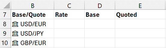
Step 1: Define Currency Pairs

In our worksheet, we type pairs like USD/EUR, GBP/JPY, etc., into a column.

Step 2: Convert to Currencies Data Type

We select the pairs, go to the Data tab, and click Currencies under Data Types. Excel transforms these text strings into linked data types powered by Refinitiv. The resulting pairs are converted to a currency data type, and get a little icon indicator:

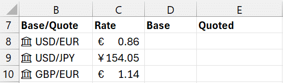
Step 3: Extract Exchange Rates

Select these currency cells, click the Insert Data icon, and choose “Price” from the list to display the current rate. Now you have the exchange rates displayed in the worksheet:

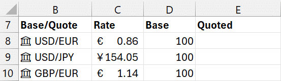
Step 4: Enter the Base Amounts

In adjacent columns, type a base amount like 100 that you’d like to convert.

Step 5: Calculate the Converted Amount

Then multiply the amount by the exchange rate to get the converted value:

=C8 * D8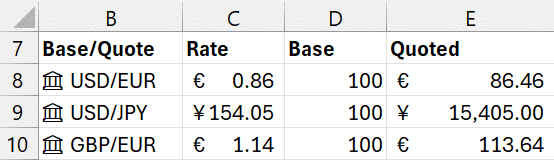

Now we have a live-updating currency conversion calculator. To refresh the rates manually, right-click on the currency icon and select Data Type > Refresh.

Method 2: Real-Time Conversion with WEBSERVICE and a Free API

In this method, we use a free API to bring conversion results directly into Excel using the WEBSERVICE function.

Step 1: Understand the API Format

A sample URL might look like this:

https://api.frankfurter.app/latest?from=USD&to=EUR&amount=100

Opening it in a browser returns a JSON result showing the converted amount and other metadata.

Step 2: Use WEBSERVICE() in Excel

In Excel, write the API URL into one cell (e.g., C4), and use the WEBSERVICE function. If you aren’t familiar with it, here is a short summary:

WEBSERVICE Function

Returns: Data from a specified web service as a text string.
Signature: =WEBSERVICE(url)
Arguments:

• url (required): The URL of the web service to retrieve data from.

We write the following formula to pull the data from the URL stored in C4:

=WEBSERVICE(C4)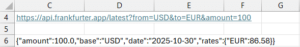

Step 3: Make the Amount Dynamic

Instead of passing the amount, 100, via the URL, let’s remove it from the base url and concatenate the user’s input value into the URL for live updates:

=WEBSERVICE(C4 & D8)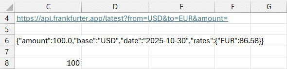

Where C4 is the API base URL and D8 is the amount entered by the user.

Step 4: Extract Just the Quoted Amount

If using the COPILOT function (requires a Copilot license), we can use natural language. If you aren’t familiar with this function, here is a quick explainer first:

COPILOT Function

Returns: AI-generated response based on prompt and referenced data, as single value or dynamic array.

Signature: =COPILOT(prompt_part1, [context1], [prompt_part2], [context2], ...)

Arguments:

• prompt_part (text, required): Describes task/question for AI; alternates with contexts.
• context (grid reference, optional): Cell/range providing data for AI.

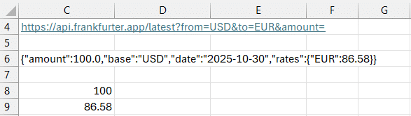
We can use it in C9 in our worksheet like this:

=COPILOT("get the EUR amount from the text string", C6)

Now, the converted amount is shown in the formula cell (C9):

If we want to use it with functions that don’t require a COPILOT license, we can a bunch of different functions, including MID, LEN, FIND, SEACH, TEXTBEFORE, TEXTAFTER and others. In this case, I’ll use TEXTSPLIT and INDEX to extract it.

If you aren’t familiar with these functions, here are some quick explainers first.

TEXTSPLIT Function

Returns: An array of substrings split by delimiters into columns and/or rows.

Signature: =TEXTSPLIT(text, col_delimiter, [row_delimiter], [ignore_empty], [match_mode], [pad_with])

Arguments:

• text (required): Text string to split.
• col_delimiter (required): Character(s) delimiting columns.
• row_delimiter (optional): Character(s) delimiting rows.
• ignore_empty (optional): TRUE to ignore empty segments (default FALSE).
• match_mode (optional): 0 for exact match, 1 for wildcards, 2 for case-sensitive (default 0).
• pad_with (optional): Value to fill uneven arrays (default empty string).

INDEX Function

Returns: A value or reference from a specified position in a range or array.

Signature: =INDEX(reference, row_num, [column_num], [area_num])

Arguments:

• reference (required): Range or array to search.
• row_num (required): Row position in the reference.
• column_num (optional): Column position in the reference.
• area_num (optional): Selects which range in multi-range reference (default 1).

Now, we can combine them as follows:

=INDEX(TEXTSPLIT(C6, ":", "}"), 1, 6)

Wrap it in VALUE() to convert from text to number if needed.

VALUE Function

Returns: A number converted from a text string that represents a number.
Signature: =VALUE(text)
Arguments:

• text (required): The text string enclosed in quotation marks that you want to convert to a number.

We wrap the VALUE function around our C9 formula as follows:

=VALUE(INDEX(TEXTSPLIT(C6, ":", "}"), 1, 6))

Method 3: Import Currency Data with Power Query

Power Query allows us to load and transform full currency tables from a web source. This method is more advanced but extremely powerful for building dynamic dashboards.

Step 1: Connect to the API

Go to Data > Get & Transform > From Web, paste in a URL such as:

https://open.er-api.com/v6/latest/USD

Click Connect, and Power Query will launch with all the returned structured data.

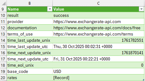
Step 2: Load Metadata

Select the top-level record, convert it to a table, then click Close & Load To > Table > Existing Worksheet.

Step 3: Extract Exchange Rates

Right-click the original query and create a Reference. Drill into the “rates” record, convert to a table, then Close & Load to your sheet.

Step 4: Use Formulas to Build Conversion Calculator

We can then pull the exchange rate for any currency we need, and apply it to the base rate amount. Use your favorite lookup function to do so. Here, I’ll use XLOOKUP. If you aren’t familiar with it:

XLOOKUP Function

Returns: Searches a range or array and returns the item corresponding to the first match found, or the closest approximate match if no match exists.
Signature: =XLOOKUP(lookup_value, lookup_array, return_array, [if_not_found], [match_mode], [search_mode])
Arguments:

• lookup_value (required): The value to search for; if omitted, returns blank cells found in lookup_array.
• lookup_array (required): The array or range to search.
• return_array (required): The array or range to return.
• if_not_found (optional): Text to return if no valid match is found; if omitted, returns #N/A.
• match_mode (optional): Specifies match type: 0 for exact match (default), -1 for exact or next smaller, 1 for exact or next larger, 2 for wildcard match.
• search_mode (optional): Specifies search mode: 1 for first-to-last (default), -1 for last-to-first, 2 for binary ascending, -2 for binary descending.

We use XLOOKUP to retrieve the rates (shown in G) for the currencies stored in F:

Finally, we multiply the amount by the rate to get the converted amount.

We can refresh exchange rates anytime with Data > Refresh All.

Quick Summary

We explored three methods for getting live exchange rates and doing currency conversion right inside Excel:

• Currencies Data Type: Great for quick setups and Excel-native integrations that update dynamically.
• WEBSERVICE with Free API: Flexible and works directly in cells, but requires text parsing.
• Power Query: Ideal for recurring workflows and importing full exchange rate tables.

Thanks for following along! We hope this guide helps streamline your foreign exchange workflows directly within Excel. Keep exploring and happy calculating!

Download the Example Excel File

FAQs about Exchange Rates in Excel

Q1: How to update the Currencies Data Types?

Right-click and choose “Data Type > Refresh” to update manually.

Q2: Is the WEBSERVICE function available in all Excel versions?

No, it’s primarily supported in Excel for Windows. Office for Mac may not fully support it.

Q3: What is the source of the exchange rates in linked data types?

Excel pulls this data from Refinitiv, a trusted financial data provider.

Q4: Can I change the base currency in a data type?

Yes, simply change the pair in the format “USD/EUR” to another combination, and Excel updates the data.

Q5: Is Power Query better than WEBSERVICE?

Power Query is better for structured and repeating tasks, while WEBSERVICE is easy for ad hoc or individual conversions.

Q6: Are these APIs free?

Yes, the apis illustrated in this post are free and do not require authentication.

Q7: How often can I refresh data using Power Query?

You can refresh on demand or set up scheduled refreshes if using Power BI or Excel Online with Power Automate.

Q8: Can I combine exchange data with other finance models in Excel?

Absolutely. Use exchange rates in budgeting, forecasting, and international sales analysis.

Q9: What if the API changes or breaks?

Switch to another API provider, such as Open Exchange Rates or CurrencyStack. Read their documentation for endpoints.