Unpivot with Power Query: Transform Wide Data into Tidy Tables

Wide data with multiple amount columns might look like a report, but it fights analysis every step of the way. Power Query’s Unpivot Columns command fixes that by collapsing those side-by-side month columns into a single, clean Amount column. The result is a tidy tabular structure that PivotTables, charts, and formulas all love. In this tutorial, we walk through three exercises: a basic unpivot from an Excel Table, a more advanced scenario with actual date headers and a totals row, and finally a demonstration of just how flexible tabular data can be once it is properly structured.

Exercise 1: Basic Unpivot from an Excel Table

Let’s say we have a dataset that looks like this:

The table has one row per account and a separate column for each month. That works fine as a printed report, but it is a nightmare for analysis. What we really want is one row per account per month, with a single Amount column. That is exactly what unpivoting gives us.

Because this is an official Excel Table (created with Ctrl+T), the month headers are stored as text values, not real dates. That is an important detail we will revisit in Exercise 2. For now, we select any cell in the table and go to Data, then Get & Transform Data, and click From Table/Range. Power Query opens immediately.

Inside the Power Query Editor, we select the Jan column, hold Shift, and click the Jun column. That selects all six month columns at once. Then we go to Transform and click Unpivot Columns. Power Query collapses those six columns into two: Attribute (containing the month names) and Value (containing the amounts). We double-click Attribute and rename it Month, then double-click Value and rename it Amount.

We hit Enter, and bam: 36 clean rows, one per account per month. We then go to Home, Close & Load To, choose Table in an existing worksheet, pick a cell, and click OK.

Future-Proofing the Query

There is one more thing we need to handle. When Power Query recorded our steps, it hardcoded the month column names inside a Changed Type step. That means if a July column shows up next period, the query will break. To fix this, we double-click the query to edit it, go to View, and click Advanced Editor.

We can see the problem clearly. The Changed Type step lists Jan, Feb, Mar and so on explicitly. We close the editor, click the Changed Type step in the Applied Steps panel, and delete it. We repeat that for any other Changed Type step that lists specific month columns. After those steps are removed, we set data types manually on the remaining steps (Account and Month as Text, Amount as Whole Number). Now the query is flexible and will handle new month columns automatically when we refresh.

Exercise 2: Unpivot with Date Headers and a Totals Row

Now it is time to make things more interesting. Consider the following worksheet:

This one has real date values in the column headers, a Total row at the bottom, and a Total column on the right. It is also a plain range, not an Excel Table. If we try to load it with From Table/Range, Power Query immediately offers to convert it to a table, which would turn those real dates into text. We click Cancel.

The trick here is to name the range first. We select the entire data range, click the Name Box in the upper-left corner, type data, and press Enter. Now when we go to Data and click From Table/Range, Power Query loads the named range directly without converting it to a table. The date headers stay intact.

Cleaning Up in Power Query

Once inside Power Query, we have a few cleanup tasks before we can unpivot. First, the column headers have not been promoted yet. We click Use First Row as Headers on the Home tab. That pushes the Dept, Account, and date values up into the header row.

Next, we filter out the Total row by clicking the Dept column drop-down and unchecking Total. Then we select the Total column and press Delete to remove it. Now our data is clean and ready to unpivot.

We select the first date column, hold Shift, and click the last date column. Then we go to Transform and click Unpivot Columns. We rename the Attribute column to Month and the Value column to Amount. But there is one more detail: the Month column is still text at this point. If we try to convert it straight to Date, we get an error because the underlying value also includes a time component.

No worries. We convert it to Date/Time first, then convert Date/Time to Date. Power Query asks whether to replace the current step or add a new one. We choose Add New Step. We hit Enter, and bam: a clean Date column with values like 1/31/2030.

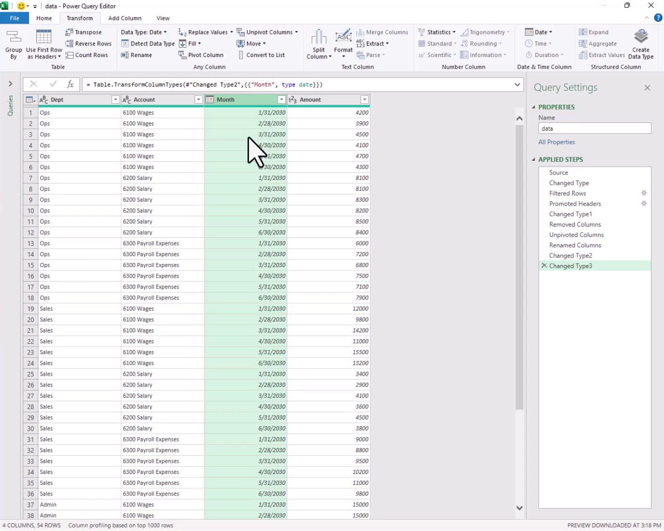
We once again visit the Advanced Editor to remove any Changed Type steps that have hardcoded month column names. After that, we head to Home, Close & Load To, and send the result to an existing worksheet as a table.

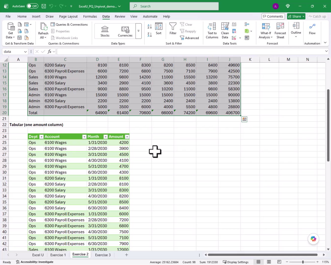
The result is a four-column table with one row per department-account-month combination. Clean, tidy, and analysis-ready.

Exercise 3: Why Unpivot? Separating Data from Reports

So, how can we demonstrate why all that unpivot work is worth it? Well … with PivotTables. When our data is in a tabular structure, we can build an almost unlimited variety of reports from a single source. We select a cell in our data table, go to Insert, and click PivotTable. We place it on an existing worksheet and click OK.

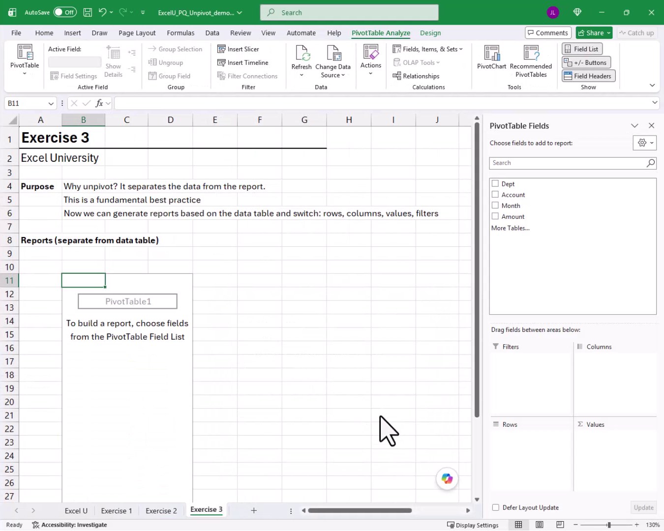
From here, we can drag Account to Rows and Amount to Values for an account-level summary. We can swap Dept in place of Account with a single checkbox click. We can drag Month into Columns to recreate the original wide-format report view.

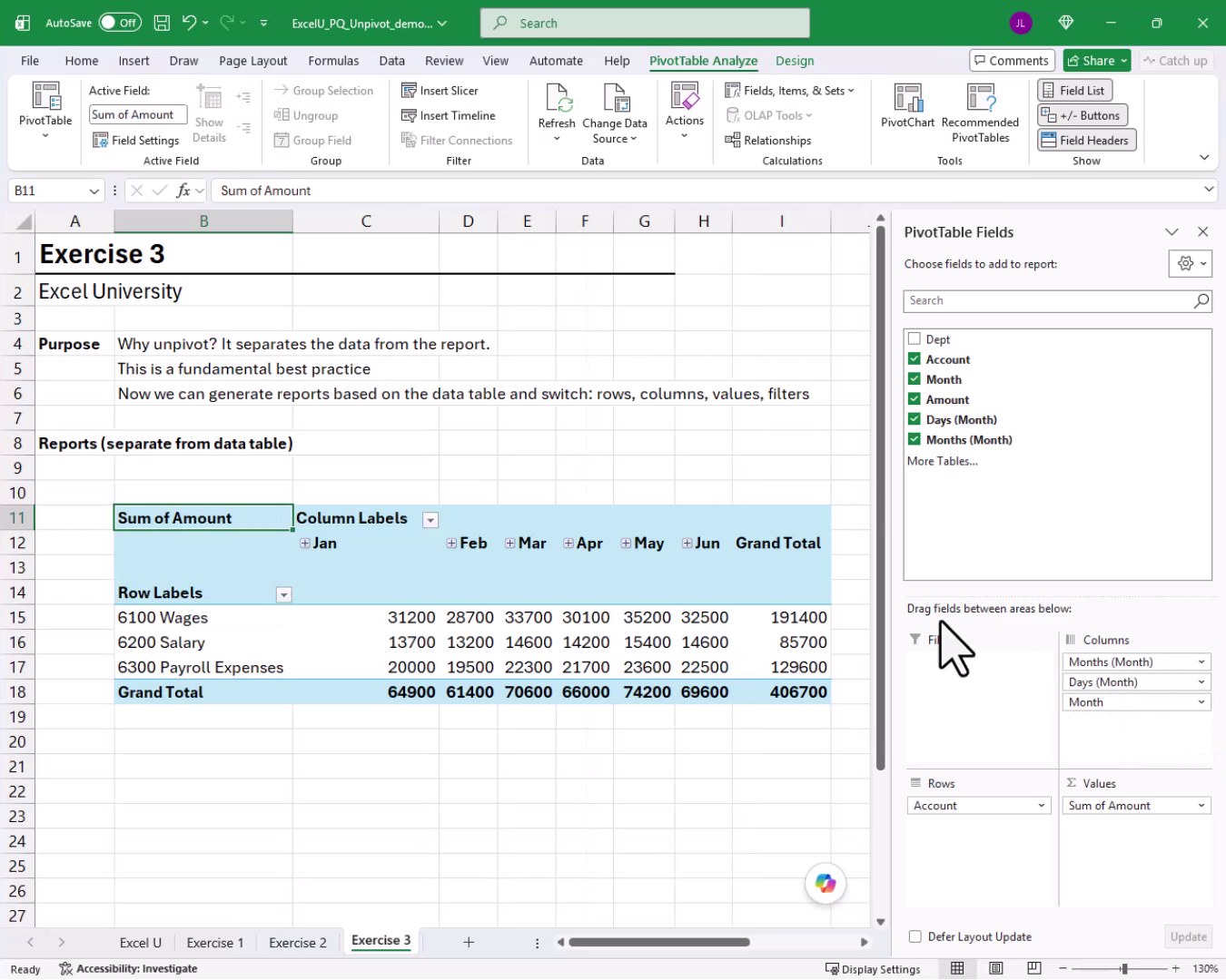
And because our Month column contains REAL dates (not text), Excel’s grouping feature works perfectly. We right-click a month label, choose Group, select Quarters, and click OK. We fill the formula down, and bam: a quarterly summary report with almost no effort.

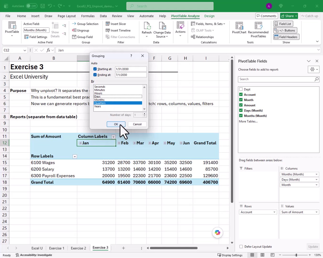
This is the fundamental best practice. Data lives in one place, in a clean tabular format. Reports are generated FROM the data, not embedded IN it. Separating the two makes everything easier to maintain AND easier to build upon.

Summary

In this tutorial, we covered how to use Power Query’s Unpivot Columns command to transform wide, report-style data into clean tabular tables. In Exercise 1, we unpivoted a standard Excel Table with text month headers. In Exercise 2, we tackled a plain named range with real date headers, a Total row, and a Total column, walking through the extra cleanup steps required. In Exercise 3, we showed exactly why tabular data is worth the effort, spinning up multiple PivotTable layouts and grouping by quarter in seconds. The unpivot workflow is one of the most valuable tools in any Excel professional’s toolkit.

If you have any suggestions, improvements, alternatives, or questions, please share by posting a comment below … thanks!

Sample File

FAQs

What does unpivot mean in Power Query?

Unpivoting converts a wide table with multiple value columns (like one column per month) into a tall table with a single value column and a new attribute column that holds the original column headers. For example, six month columns become two columns: Month and Amount.

Why is tabular data better than wide data for analysis?

Tabular data keeps one fact per row, which is the structure that PivotTables, charts, and functions like SUMIFS all expect. Wide data mixes structure with content, making it hard to filter, group, or aggregate without manual workarounds.

What is the difference between Unpivot Columns and Unpivot Other Columns in Power Query?

Unpivot Columns unpivots only the columns we explicitly select. Unpivot Other Columns unpivots everything EXCEPT the columns we select, which is often more future-proof because new columns added to the source will automatically be unpivoted without any query edits.

Why should we delete the Changed Type step when future-proofing a query?

Power Query’s auto-generated Changed Type step lists every column name explicitly. If new columns appear in the source (like a July column), the query will either error out or ignore them. Deleting that step removes the hardcoded column list so new columns flow through without breaking anything.

Why do we name the range before loading it into Power Query?

When we click From Table/Range on a plain range, Power Query tries to convert it to an Excel Table first. That conversion turns real date values in headers into text, which breaks date-based operations later. Naming the range lets Power Query load it directly without that conversion.

Why do we need to convert the Month column to Date/Time before converting it to Date?

When date values come through as text after unpivoting, they often include a time component (like 1/31/2030 12:00:00 AM). Power Query cannot convert that text string directly to a Date type. We must go through Date/Time first, which correctly parses the full timestamp, and then convert to Date.

Does the Unpivot Columns command work on data that is not in an Excel Table?

Yes. As we showed in Exercise 2, we can load a plain named range into Power Query and use Unpivot Columns just as we would with a table. The key is to name the range first so Power Query does not force a table conversion.

What happens when we add new rows or columns to the source data?

For new rows, we simply right-click the results table in Excel and click Refresh. The new rows flow through the query automatically. For new columns (like a new month), the query will include them automatically as long as we removed the hardcoded Changed Type steps that listed specific column names.

Can we use PivotTable grouping on the Month column after unpivoting?

Yes, but only if the Month column contains real date values, not text. When dates are stored as actual dates (as we set up in Exercise 2), PivotTable grouping lets us summarize by month, quarter, or year with just a few clicks. Text-based month columns like those from Exercise 1 do not support this feature.

Is Power Query available in all versions of Excel?

Power Query is built into Excel 2016 and later on Windows. It is also available in Excel for Microsoft 365. Excel 2010 and 2013 users can install it as a free add-in from Microsoft. Power Query is not available in Excel for Mac in the same full-featured way it is on Windows.