Turn a Table of Events into a Graphical Calendar

Today, we’re tackling the following question: How do you create a calendar that can show multiple events per day in Excel? We’re going to transform a simple table of events into a dynamic, graphical calendar. Let’s dive right in!

Objective

In summary, we have a list of events stored in a Table named Table1, like this:

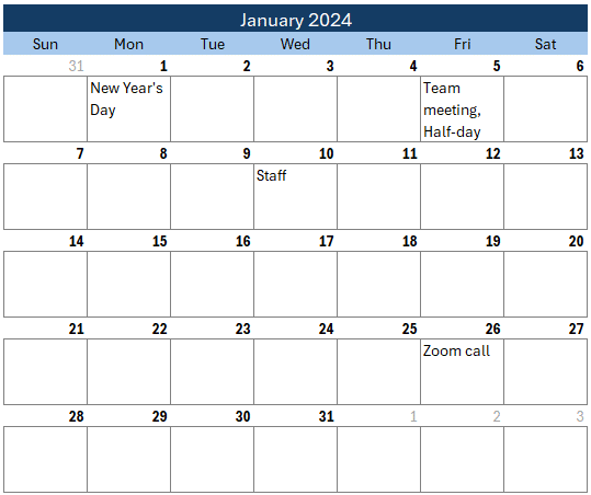
We want to dynamically pull those events into a calendar like this:

First, let’s get familiar with the functions we’ll be using.

Exercise 1: Getting Familiar with Functions

Before we build our calendar, let’s warm up with some key functions we’ll be using.

1. SEQUENCE Function

The SEQUENCE function generates a sequence of numbers. Here’s how to use it:

• Formula: =SEQUENCE(rows, columns, start)
• Example: =SEQUENCE(1, 5, 10)
  • This creates a sequence starting at 10, with 1 row and 5 columns.

2. WEEKDAY Function

The WEEKDAY function returns the day of the week for a given date.

• Formula: =WEEKDAY(date)
• Example: =WEEKDAY(“2024-01-01”)
  • 1 is Sunday; 2 is Monday; and so on.

3. EOMONTH Function

The EOMONTH function returns the last day of the month for a given date.

• Formula: =EOMONTH(start_date, months)
• Example: =EOMONTH(“2024-01-01”, 0)
  • This returns January 31, 2024.

4. ARRAYTOTEXT Function

The ARRAYTOTEXT function converts an array or range of cells to a comma-separated list.

• Formula: =ARRAYTOTEXT(array)
• Example: =ARRAYTOTEXT(A1:A5)
  • This returns a comma-separated list of the values in cells A1 to A5.

5. FILTER Function

The FILTER function returns an array that meets specified criteria.

• Formula: =FILTER(array, include, [if_empty])
• Example: =FILTER(A1:A10, B1:B10=”Category1″, “”)
  • This returns the values in A1:A10 where B1:B10 equals “Category1”.

With our functions identified and summarized, it is time to use them to build our calendar!

Exercise 2: Building the Calendar

Now, let’s combine these functions to build our calendar.

We are basically going to create several pairs of formulas. The first row in each pair will compute the dates in a week (highlighted in yellow below). The second row in each pair will retrieve the events from the calendar for each date (circled in red below).

Once we have this pair of formulas set up, it is easy to replicate them for the remaining weeks.

Step 1: Generate a Row of Dates

We’ll use the SEQUENCE function to create a row of dates for the first week of the month.

Let’s enter the date the calendar should start in a cell like C6:

We can use the following formula to create a row of seven dates that begin on the date in C6:

=SEQUENCE(1, 7, C6)

This generates dates from January 1 to January 7, 2024.

Note: depending on the formatting in the cells, the dates may look like these date serials, which represent the underlying dates:

It is easy to select these cells and apply a date format so they look more like dates:

Now, we want to ensure that this row of dates begins on a Sunday to align with our graphical calendar layout. So, we need to adjust the first date based on the weekday in C6. We can use the WEEKDAY function to do so with the following update to our formula:

=SEQUENCE(1, 7, C6 - WEEKDAY(C6) + 1)

Now the first date is a Sunday:

Step 2: Populate the Calendar

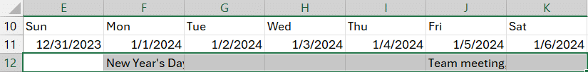
For the next row, we’ll use the FILTER function to retrieve all of the events for each day in the cell above (E11) from our events Table named Table1:

=ARRAYTOTEXT(FILTER(Table1[Event], Table1[Date]=E11, ""))

We can fill this formula right, and bam:

Note: in the next exercise, we’ll talk through formatting options for the calendar.

Step 3: Repeat for Subsequent Weeks

We can use similar formulas to create the remaining weeks. For each week row, the SEQUENCE function should start at the last date in the previous week + 1. The FILTER function can be copy/pasted to retrieve the events. We basically end up with something like this:

Now let’s talk through some formatting options.

Exercise 3: Cosmetics

Formatting the Calendar

1. Month Header: The month header can be a simple formula that points to the calendar start cell C6, and can be formatted as follows:
   • Select the date cell and cells to the right to span the week
   • Format Cells > Alignment > Horizontal > Center Across Selection
   • Format Cells > Number > Custom: mmmm yyyy
   • Bold text and a background color
2. Day Labels: Center-align day labels and apply a light background color
   • Format Cells > Alignment > Center
3. Date Cells: Display only the day number
   • Format Cells > Number > Custom: d
4. Conditional Formatting: Highlight dates within the current month
   • Select all date rows
   • Conditional Formatting > Highlight Cell Rules > Between
   • From: calendar start date =C6
   • To: end of month =EOMONTH(C6, 0)

Adjusting Row Heights and Wrapping Text

1. Row Height: Set a consistent row height for event rows.
   • Right-click rows > Row Height > 45
2. Wrap Text: Ensure text in event cells wraps to fit within the cell.
   • Format Cells > Alignment > Wrap Text
3. Borders: Add borders to event cells for better readability.
   • Format Cells > Border > Outline and Inside

Now our calendar looks something like this:

Dynamic Updates

Your calendar is now fully dynamic! Changing the start date updates all dates and events accordingly. You can add additional events to the events Table and changes are instantly reflected in the calendar.

Conclusion

And there you have it! We’ve built a dynamic, multi-event calendar using Excel’s powerful functions. This calendar is perfect for tracking events, appointments, and more. If you have any questions or comments, feel free to leave them below. Thanks for joining me, and have a great day!

Sample File

FAQ:

Q. Can I add more events to the table?

Yes, simply add more rows to your events table, and the calendar will update automatically.

Q. How do I change the start date of the calendar?

Update the start date in the calendar start cell (C6 in this case).

Q. What if there are no events on a particular day?

The FILTER function handles this by returning an empty cell if no events match the date.

Q. How can I customize the look of my calendar?

You can customize fonts, colors, and cell styles using Excel’s formatting options.

Q. Can this calendar handle a different week start day?

Yes, you can start the calendar on any week day, for example Monday, but updating the first SEQUENCE function accordingly.

Q. Can I use this calendar for different years?

Absolutely! Adjust the start date to the desired year, and the calendar will update accordingly.

Q. Is it possible to show events from multiple categories?

Yes, modify the FILTER function to include multiple categories as needed.

Q. How do I print the calendar?

Set your print area to include the calendar range and adjust the page layout for best results.

Q. Can I share this calendar with others?

Yes, save the Excel file and share it with others, or use Excel Online for collaborative editing.