Last Date in Column

Hello and welcome to our latest tutorial! Today we’re diving into a common Excel challenge: finding the last date in a column. This is especially useful if you add rows to your data regularly. Let’s explore three different exercises to solve this problem.

Video

Tutorial

Exercise 1: Using the TAKE Function in a Table

Step-by-Step Guide

In this first exercise, we’ll assume your data is stored in a Table (created with the Insert > Table or Ctrl+T command). This makes our task straightforward, especially if you have a newer version of Excel that includes the TAKE function.

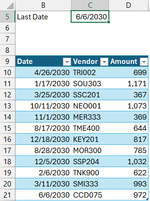
Set Up Your Table: Ensure your data is stored in a table. If it isn’t, select your data range and press Ctrl+T to convert it into a table. By default, Tables are formatted with blue/white banded rows and should look something like this:

There are a couple of different functions we can use to retrieve the last date in the date column. Some versions of Excel include the TAKE function, and others don’t. So, let’s walk through options.

TAKE Function

If your version of Excel supports the TAKE function (which you can determine by typing =TA into a cell and seeing if TAKE appears in the list that appears). If so:

• Enter the formula =TAKE(Table1[Date], -1)
• This formula tells Excel to take the last row in the Date column of your table
• Update Table1[Date] to reflect your table name (found in the Table > Table Name field) and the column that contains the date

That’s it:

As you enter new data rows to your table, the formula will update and retrieve the date from the last row of the table.

Now, if your version of Excel doesn’t support the TAKE function, you can use a combination of the INDEX and ROWS functions (which will be in your Excel because these have existed for decades).

INDEX and ROWS Functions

1. Set Up Your Table: Ensure your data is in a table format.
2. Use the INDEX and ROWS Functions:

• Enter the formula =INDEX(Table1[Date], ROWS(Table1[Date]))
• This formula calculates the total number of rows in the Date column and returns the value from the date column in that row

Both methods will return the last date in your Date column, even as new table rows are added.

Exercise 2: When Data is Not in a Table

In the second exercise, we tackle a scenario where your data isn’t stored in a Table. Here, we’ll use the INDEX and MATCH functions.

Step-by-Step Guide

1. Set Up Your Data: Ensure your dates are listed in a column, say column B.
2. Use the INDEX and MATCH Functions:

• Enter the formula =INDEX(B:B, MATCH(0, B:B, -1))
• This formula finds the last date value in Column A (assuming all values in Column A are dates).

This formula will update to show the last date in the column (meaning, the furthest down the worksheet). Even as new dates are entered, the formula will continue to update to retrieve the last date in the column.

Exercise 3: Finding the Date Range

Sometimes, you might not need the last date (the one furthest down the worksheet) but instead, the earliest or latest date value. In this exercise, we’ll use the MIN and MAX functions to find the earliest and latest dates in your column.

Step-by-Step Guide

Set Up Your Data: Ensure your dates are in a single column.

Find the Minimum Date:

• Enter the formula =MIN(B:B)
• This will return the earliest date in your column

Find the Maximum Date:

• Enter the formula =MAX(A:A)
• This will return the latest date in your column.

Now you have the full range of dates, from the earliest to the latest, included in your dataset. For example, if your dates range from January 17 to December 18, these formulas will display those dates.

Conclusion

Finding specific date values in a column, whether your data is in a Table or not, is a task you can handle easily with the right functions. We covered the TAKE, INDEX, ROWS, MATCH, MIN, and MAX functions to give you a variety of tools to use based on your Excel version and data structure.

Feel free to leave any questions or comments below … thanks!

Sample File

FAQ

Q: What if my version of Excel doesn’t support the TAKE function?
A: You can use the INDEX and ROWS functions as an alternative to find the last date in your column.

Q: How do I convert my data range into a Table?
A: Select your data range and press Ctrl+T to convert it into a table. This makes it easier to manage and analyze your data.

Q: What if my dates are stored in a different format?
A: Ensure your dates are recognized as date values in Excel. You can use the DATEVALUE function to convert text dates into proper date values.

Q: Can I use these functions in Google Sheets?
A: While some functions like TAKE might not be available, you can use similar functions like INDEX, ROWS, and MATCH in Google Sheets to achieve the same results.

Q: How do I handle empty rows in my data?
A: The formulas provided will still work even if there are empty rows, as long as the date values are correctly formatted.

Q: Can these methods handle dynamic data ranges?
A: Yes, using a Table ensures your formulas update automatically as you add or remove data.

Q: What if my data includes time stamps along with dates?
A: The formulas will still work, but you might need to format the result to display only the date portion.

Q: How do I troubleshoot errors in these formulas?
A: Ensure your data is correctly formatted and there are only dates in the column (eg, no text values or negative numbers).