Treasure Maps 2

This is the second post in the Treasure Maps series, where we are discussing various ways to implement mapping tables. In the first post, we covered SUMIFS. In this post, we’ll talk about Power Query.

Overview

Let’s say we have a list of transactions in a CSV file, like this:

We would like to use the data to build a report like this:

Since the transaction labels (Acct ID 1000, 1001, 1002, …) and the report labels (Cash and Cash Equivalents, Inventory, …) are different, we need a way to translate them. So, we create a mapping table, like this:

We could save the mapping table just about anywhere, for example a CSV file, Excel workbook, or Access database. In this case, we’ll keep things simple and save it to a CSV file.

Now, let’s see how to connect the dots with Power Query.

Video

Narrative

We will accomplish this in three steps:

• Load the tables
• Merge
• Build the report

Let’s jump right in.

Load tables

We need to load our transaction and mapping tables into Power Query. We’ll start with the transaction table.

Transactions

The first thing we need to do is to pull the transactions into Power Query. Since our transactions are stored in a CSV file, we’ll use the Data > Get Data > From File > From Text/CSV and then browse to our transactions file.

Note: If your transactions are elsewhere, you would use the corresponding Get Data option.

We can see a preview like this:

Since our data is clean, there are no transformations needed. We can expand the Load button by clicking the down arrow and selecting Load To. In the resulting dialog, we select Only Create Connection, like this:

Note: if your data needs to be cleaned up, you would click the Transform button and make any transformations needed before loading the query to a Connection Only Query.

Since we loaded it to a connection-only query, we do not see the results in an Excel table … yet. Which is perfect. Now that the transactions are in Power Query, it is time to pull the Mapping Table into Power Query.

Map

We basically perform the same steps to retrieve the mapping table. Since our map is stored in a CSV, we can use the Get Data > From File > From Text/CSV and browse to the map file. We see the preview and once again, Load To a connection-only query.

At this point, we should have the data and map queries in our workbook. We should see them in the Queries & Connection pane, like this:

With our data and map queries in place, it is time to combine them.

Merge

To combine these two queries, we use the Get Data > Combine > Merge command. In the resulting Merge dialog, we select our data query from the top drop down and our map query from the bottom drop down, like this:

Now we need to tell Power Query how these two tables are related. If you are familiar with VLOOKUP, it is like identifying the lookup value.

In our case, the lookup column is AcctID. So we select both AcctID columns, like this:

We click OK and see the results in the Power Query editor, like this:

We click the expand button on the right side of the map column header, and select the columns we want to display … in our case, the FS Line column. The results look like this:

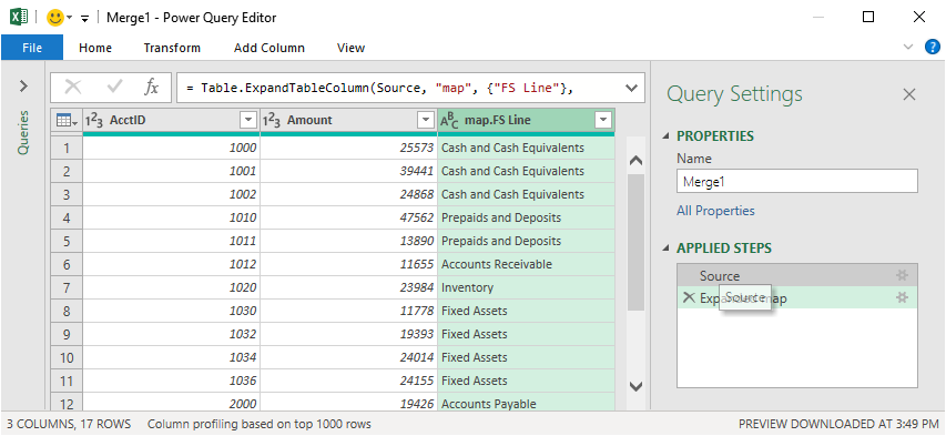
With this complete, we can use the Home > Close & Load To command, and select our destination in the resulting dialog. In our case, we’ll load the results to a Table in a new worksheet:

We click OK, and the resulting table (in this case, named Merge1) is displayed in our worksheet:

Now all that remains is to build our report.

Report

We have options for which type of report to use to summarize the data. In this post, we’ll use a formula-based report and revisit the SUMIFS function discussed in the first post in the series.

Here is our report layout:

We can write the following formula into cell G12:

=SUMIFS(Merge1[Amount],Merge1[FS Line],F12)

And then fill that formula down … bam:

Yay … we did it!

Conclusion

To update the report in future periods, we simply right-click the green results table (eg, Merge1) and select Refresh. Power Query will retrieve the updated transactions file as well as any changes made to the map. Provided there are no new FS Lines and that any new accounts are added to the map, we are good to go.

But, what if there are new FS Lines added to the map? With this formula-based solution, we would need to insert them manually into our report. But, in the next post, we’ll look at how to use a PivotTable instead of formulas and address that issue 🙂

Sample file

Note: I combined the report and data into a single file for simplicity