Treasure Maps 1

This is the first post in the Treasure Maps series, where we’ll be discussing the treasure (efficiency) that can be achieved by using mapping tables.

Let’s review the big picture before jumping into the mechanics.

Let’s say we export some data from a system, and it looks something like this (we’ll call this Point A):

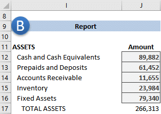
And, let’s say we want to do something with the data that requires DIFFERENT labels. For example, perhaps we would like to get the numbers into a report like this (we’ll call it Point B):

Since the LABELS between them are DIFFERENT, how do you get from Point A to Point B?

The labels are different (AcctName versus the report labels), so we can’t simply use a lookup function like VLOOKUP. One option is to write formulas that point to the individual cells. Perhaps something like this:

=B1+B2+B3

Then, the next cell in the report would point to different cells, perhaps like this:

=B4+B5

There are a couple of problems with this approach. First, each cell in report B requires a custom formula … that is … we can’t just fill the formula down. This requires us to write a unique formula for each cell in the report. This isn’t very efficient.

Second, this approach is fragile. Meaning if someone sorts the data in A, report B will break. Or, if the order of the data changes next month when we paste updated data, report B will break.

Rather than taking such a circuitous and dangerous route, we can use a map. A map will help us get from point A to point B more efficiently. A map simply defines the label translation between two tables, like this:

I like to think of this as a treasure map, because it helps us discover the treasure of efficiency!

Implementation

There are many ways to implement such a map (aka, mapping table, transformation table, or lookup table). In this series, we’ll look at three ways to implement mapping tables. Specifically, we’ll discuss:

• SUMIFS
• Power Query
• Power Pivot

In this post, we’ll use SUMIFS to implement our mapping table.

Video

SUMIFS

SUMIFS is a conditional summing function. If you haven’t explored it much, feel free to review these SUMIFS posts as I’ve written about it quite a bit. From a high level, it allows us to add up a column of numbers and only include the rows that meet one or more conditions. The basic syntax is this:

=SUMIFS(sum_range, criteria_range1, criteria1, ...)

With this implementation, we would basically use SUMIFS to pull the numbers from the source data into the map, and then again to pull the numbers from the map into the final report. Although the text below is tiny, here is an image that provides the general idea:

Now, let’s get to work. We’ll start by getting the numbers from the data source into the map.

Data > Map

Let’s say the data is stored in a table named Table1, like this:

We then create our basic map and store it in a table named Table2, like this:

We need to bring the amount values from Table1 into the map. We can use SUMIFS to populate the map’s Amount column, like this:

=SUMIFS(Table1[Amount], Table1[AcctName], [@AcctName])

We hit Enter, and bam:

With that done, all we need to do is get the numbers from the map into the report.

Map > Report

Now that we have the values in our map (Table2), we need to get them into our report:

To pull the values from the map into the report, we’ll use SUMIFS. We can write the following formula into J12:

=SUMIFS(Table2[Amount],Table2[FS Line],I12)

When we copy the formula down … bam:

Now, the nice thing is that when our data table is updated with different transactions, they all flow through to the report automatically. When we have a new account, we can add it to the mapping table. And if we have a new FS Line, we can add it to the report.

Conclusion

This is one of many possible ways to implement a mapping table. In the second post, we explore another option that uses Power Query.

Sample File