Sort a PivotTable with a Custom List

In this post, we’ll talk about how to use a custom list to automatically sort a PivotTable. By default, a PT is initially displayed in alphabetical order by the row labels. But, what if that isn’t what we want? Well, we can always manually sort each time we create a PT. But, there is a faster way for common sorts that uses a custom list … let’s check it out.

Objective

Let’s cover our objective. Our company has four regions, North, South, East, and West. Every person at our company is used to seeing all company reports showing the regions in that exact order (North, South, East, West). If we delivered a report with the regions in a different order, there would be trouble. But, when we create a PivotTable, it is initially displayed in alphabetical order, like this:

So, every time I build a report, I have to click-and-drag the regions into the correct order as shown below.

But, that is an extra step that is unnecessary when we use a Custom List.

Details

We’ll tackle this report in two steps:

• Define the custom list
• Build the report

Let’s check it out.

Define the custom list

To define the custom region list, we just head to File > Options. In the resulting Excel Options dialog, we click Advanced and scroll down to the Edit Custom Lists button.

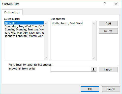
In the resulting Custom Lists dialog, we just type in our regions separated with commas into the List entries box, as shown below.

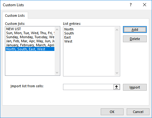
When our list is entered, click the Add button, and the list is added as shown below.

With our custom list added, it is time to build our report.

Note: the custom list is stored in your Excel Application, not in the workbook. This means that it will be applied to new PivotTables in all of your workbooks.

Build the report

To build the report, we select any cell in the data table and use the Insert > PivotTable command. We insert the Region field into the Rows area, and the Amount field into the Values layout area.  Yes … it worked!

Notes: (1) if you built the PT before setting the custom list, you’ll just need to refresh the PT and do an A>Z sort (2) if it doesn’t seem to be working, double-check that the PivotTable Options > Totals & Filters > Use Custom Lists when sorting checkbox is checked.

If you have any other fun PT tips, please share by posting a comment below…thanks!

Sample File

• CustomListPT.xlsx
• Note: the sample file includes the data, but not the PivotTable because custom lists are saved within the Excel application not in Excel workbooks.