Edit PivotTable Values

In this post, we’ll talk about how to edit the value in a PivotTable cell. Wait…what!? I’ve been using PTs for a long time, and, I’ve always received an error when I try to edit the value in a PivotTable cell. Yes, we’ve been able to edit the label cells, but, not the value cells. In this post, we will edit a PT value cell and the PT totals will update accordingly.

Objective

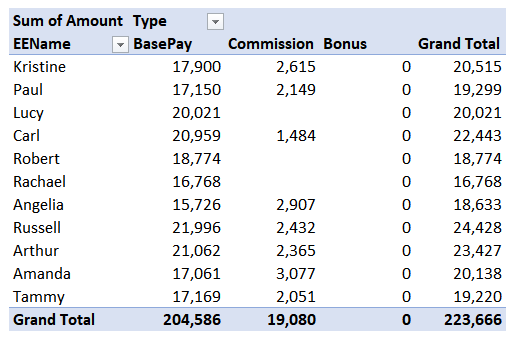
Before we get to it, let’s discuss our objective. We have a basic PT. We would like to add an Input column so that people can enter values into the PT. We want our PT totals to update to include the entered values. For example, it is time to pay our quarterly bonus. The bonus is discretionary, not tied to a fixed equation. So, we need to enable a manager to enter an arbitrary bonus amount. As a general guideline, the manager needs to see the total wages and commission for the past quarter when determining the bonus amount. So, we export the payroll data and store it in a table. Then, we create a PivotTable to provide the totals. It looks a little something like this:

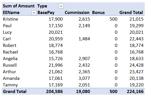
Now, we’d like to add a Bonus column so that our manager can type the bonus amounts right into the PT … AND … the Grand Total should include the bonus values. Like this:

We can do this with a traditional PT, and as a quick note, I’d like to share how I stumbled upon this capability. I was looking through the PivotTable Options dialog, and reading up on each individual checkbox. (Total nerd, I know.) Anywho, I saw an option called “What-If Analysis, Enable cell editing in the values area” and I was like, what? So, I started to investigate. I did a web search which led me to mrexcel.com (thanks Bill), contexturesblog.com (thanks Deb), microsoft.com (thanks Microsoft), and others. And, what I learned was very interesting.

As far as I can tell, that specific checkbox is disabled except under limited circumstances,  including the Excel version and data source, and that it is included now for compatibility purposes. But, during my search, I discovered that there is another way to enable a user to enter values into PivotTable cells. It is by using a Calculated Item. And, this is one thing I love about Excel … it is such a big place with so much cool stuff to learn.

Now, let’s go ahead and build a PT with an input column.

Narrative

We’ll do this by performing the following steps:

• Get the basic PT working
• Add a Calculated Item
• Test it out

Let’s get to it.

Get the basic PT working

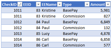
Let’s get the basic PT working first. We’ve exported the payroll data and stored it in an Excel table, a portion of which is shown below.

We select any cell in the data table, and use the Insert > PivotTable command. Then, we insert the EEName field into the Rows layout area, the Amount field into the Values area, and the Type field into the Columns area. The resulting PT is shown below.

With our basic PT done, it is time to add a Calculated Item.

Add a Calculated Item

Step 1: Select a corresponding label cell

The first step for adding a Calculated Item is to tell Excel which field the new item belongs to. The way we communicate this to Excel is by selecting a corresponding report label cell.

Let’s unpack this for a second. A Calculated Item is a PivotTable formula that operates on items within a field. A Calculated Item is NOT a Calculated Field. A Calculated Field operates on other fields. A Calculated Item operates on items within a field. This can be tricky to visualize at first, but, if you look at the source data above, you’ll notice there is a Type column (field). The Type field has two items, BasePay and Commission. We are going to create another item for the Type field by creating a Calculated Item, and we’re going to name it Bonus.

Note: We can create a Calculated Item for fields that have been inserted into the PT. This means that we are able to create a Bonus column because we have inserted the Type field into the Columns layout area. So, if we do not have a field in the columns area, we won’t be able to create a calculated item column. But, if we have a field in the Rows area, we can create a calculated item row.

With that little background on Calculated Items done, let’s press ahead with our example.

We do the first step, which is to select either the BasePay cell or the Commission cell in the PivotTable report. Here, I’ve selected the BasePay cell:

Now, we can create the Calculated Item. We click the PivotTable Tools > Analyze > Fields, Items, & Sets > Calculated Item command.

Note: if the Calculated Item option is disabled, you’ll need to select either the BasePay or Commission cell in your PivotTable report.

Step 2: Write the formula

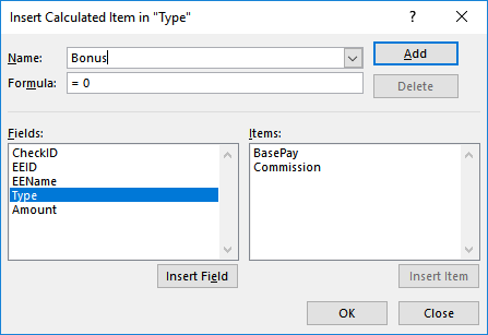
In the resulting Calculated Item dialog, we give our Calculated Item a name, Bonus, and we’ll accept the default formula =0 as shown below.

Note: to create a calculated item that actually computed a value, enter the desired formula. In this application, we want to allow users to enter a value into the PT cell, so, we don’t care about the formula and will leave it as the default =0. If we used a formula like =BasePay*.05 then it would be the default amount but a user could override the value in the PT by typing in a new bonus amount.

The PT is updated to reflect our Calculated Item, and now we have a Bonus column as shown below.

Now, it is time to test it out.

Test it out

To see if this works, we try to type in a bonus amount, 500, for Kristine. Wow … it works! Excel allows us to actually edit a PT value cell and updates the totals accordingly, as shown below.

If you’d like to check it out, the sample file below includes the calculated item.

And if you have any other PT tips, please share by posting a comment below…thanks!

Sample file

• EditPTValues.xlsx