Simulate Structured References in Named Ranges

The table feature introduced in Excel 2007 is amazing and has nearly eliminated the need to build dynamic named ranges since tables auto-expand. Beyond auto-expansion, tables offer numerous other benefits, including, structured references which allow us to refer to an area within the table, such as a specific column. In this post, we’ll examine a method to simulate structured references when using an ordinary named range.

Objective

Before we get too far, let’s be clear about our objective.

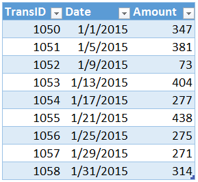
I love storing data in tables due to their special properties such as auto-expansion, structured references, and formula auto-fill. Whenever possible, I store source data in tables (Insert > Table). For example, consider the table below.

The table is named Table1. Structured table references begin with the table’s name followed by the desired area enclosed in square brackets. For example, to refer to the column named Amount in the table named Table1, the structured reference is: Table1[Amount]. So, to sum the amount column, we could use the following formula:

=SUM(Table1[Amount])

The structured reference naming system is wonderful because we can easily refer to selected regions within the table. Unfortunately, structured references don’t apply to ordinary named ranges set up with the Name Manager or the Name Box.  🙁  Fortunately, it is easy to simulate structured references with a worksheet function.  🙂

Let’s see how.

Named Ranges

Let’s begin by looking at our worksheet. The data below has not been converted to a table with the Insert > Table command. It has been assigned the name DataRange with the Formulas > Name Manager command. This name appears in the Name Box (to the left of the formula bar).

This brings us to the reason we are here: simulating the structured reference system in a named range. We want to refer to a selected area within the named range. We want to write a formula to sum the amount column.

The INDEX function will help us out. The INDEX function can return an area within a reference, such as a specific row or column. Let’s examine the INDEX function’s first three arguments.

=INDEX(reference, row_num, [column_num])

Where:

• reference is the entire reference, such as our DataRange
• row_num is the row number, or 0 for all rows
• [column_num] is the optional column number, or 0 for all columns

Let’s apply the INDEX function to sum the amount column.

We could use the following formula to sum the amount column, which is the third column in the range.

=SUM(INDEX(DataRange,0,3))

Yes…we did it! We simulated a structured table reference! This formula adds up the values in all rows in the 3rd column of the DataRange named reference.

When the column positions are static, then, using an integer value, such as 3, to identify the column works just fine. But, if the column order is dynamic or we want to write a consistent formula to fill down or right, we can get fancy and locate the column number via the column header label.

Let’s check it out.

Dynamic

If we need to, we can use the MATCH function to dynamically locate the column and then provide the corresponding column number to the INDEX function. The MATCH function returns the relative position of the matching value, and has the following syntax.

=MATCH(lookup_value, lookup_array, [match_type])

Where:

• lookup_value is the value we are trying to find, the column header
• lookup_array is where we are looking
• match_type…we’ll use 0 because we want an exact matching value

In the screenshot below, we’ve named the data range Data, and we need to write a formula in C6 to add up the amount column…and…we want to fill that same formula down to sum the values in the other columns.

The idea is to use the MATCH function to locate the column header, such as Amount, SalesTax, or Shipping, and then return the matching column number to the INDEX function. Let’s proceed one step at a time.

First, the MATCH function. We are asking the MATCH function to figure out the column number. We want to find the column label, Amount, within the first row of the Data range. We can generate a reference to the first row of the Data range with the INDEX function. Thus, the following formula entered in C6 would return 3 since the Amount header is in the third position:

=MATCH(B6,INDEX(Data,1,0),0)

Where:

• B6 is the value we are trying the find, the Amount label
• INDEX(Data,1,0) is where we are looking, the first row of the Data range
• Where:
  • Data is the reference
  • 1 is the first row
  • 0 for all columns
• 0 means we want an exact matching value

The MATCH function returns 3 since the label Amount is found in the 3rd position within the lookup range. Now, we can use the MATCH function in an INDEX function that returns the reference to the entire Amount column, as follows:

=INDEX(Data, 0, MATCH(B6,INDEX(Data,1,0),0)))

Where:

• Data is the reference
• 0 means all rows
• MATCH(B6,INDEX(Data,1,0),0) returns the 3rd column

We can then put this INDEX function inside of a SUM function and fill the formula down, as shown below.

It is nice to know that we can simulate the structured table reference naming system with worksheet functions so that we can refer to regions within an ordinary named range.

If this post has been useful, or, if you prefer another method, please share by adding a comment below!

Resources

• Sample StructuredReferenceSim
• Other INDEX posts
• Other MATCH posts
• Other Table posts