Set Default PivotTable Layout Options
If you use PivotTables often, you’ve probably wished there was a way to set default PivotTable layout options. For example, if you prefer Tabular instead of the default Compact, it sure would be nice if all new PivotTables used the Tabular layout. Well, depending on the version of Excel you have, you may in fact be able to edit the default PivotTable layout right now 🙂
I’ve prepared a video as well as a written narrative that shows the steps.
Video
Narrative
We can edit the default PT layout by using the PivotTable Options dialog. We’ll walk through these steps:
- Excel Options
- Layout Options
- PivotTable Options
Let’s get to it.
Note: the ability to edit the default PivotTable layout depends on your version of Excel. The steps below are presented with an Excel 2016 for Windows Subscription License. If you open the PivotTable Options dialog, and don’t see the buttons demonstrated below, then your current version of Excel doesn’t support these options. However, you can check out a previous post that shows how to use a macro to automatically update the value field formats.
Excel Options
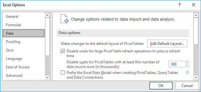
The first step is to open the Excel Options dialog, and navigate to the Data category. One way to do this is to click the File > Options command. In the Excel Options dialog, click Data and then look for the Edit Default Layout button as shown below.
This opens the Edit Default Layout dialog, which we can use to set the default layout options discussed below.
Layout Options
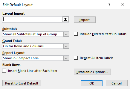
In the Edit Default Layout dialog, we have many options, as shown below.
If you already have a PivotTable with the layout options you’d like to use for the default, then you can select it and click the Import button. Otherwise, you can simply select your desired default layout options.
For example, we can control how Subtotals and Grand Totals are displayed, which Report Layout we prefer, if we’d like to Repeat all item labels, and more. Plus, we can click the PivotTable Options button to open the PivotTable Options dialog, discussed below.
PivotTable Options
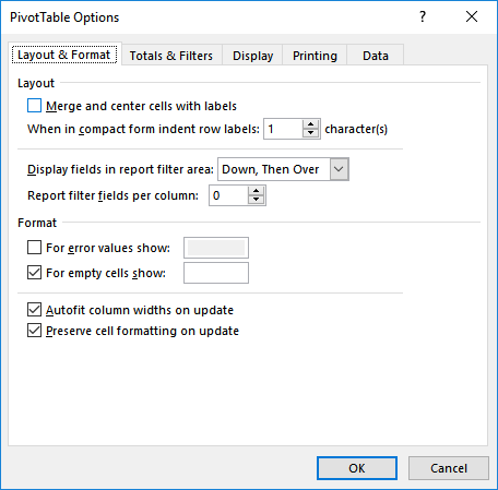
The PivotTable Options dialog is shown below.
Here we can define the default options for new PivotTables.
One option I wish would have been included is a default number format for value fields. At the time of this writing, this option isn’t available … but hopefully someday it will be. In the meantime, we can create a macro to do that, and if that would help, check out the related blog post below.
If you’d like to practice, feel free to download the sample file below.
If you have any other fun PivotTable tips, please share by posting a comment below … thanks!
Sample File
Related Blog Post
Excel is not what it used to be.
You need the Excel Proficiency Roadmap now. Includes 6 steps for a successful journey, 3 things to avoid, and weekly Excel tips.
Want to learn Excel?
Our training programs start at $29 and will help you learn Excel quickly.


Great Tip. Thank you.
Thanks, Jeff!
I don’t have the Data menu available under Excel Options. Is there a way to turn that option on?
This option depends on your version of Excel, and, to my knowledge can’t be added or turned on in versions that don’t have it built-in.
Sorry about that!
Thanks
Jeff
I can’t find a prior post that I saw. I have a Pivot table that will have no data in certain months and want to use a reference based off the month number,