Rows of Dependent Drop Downs

When working with drop down lists in Excel, creating dependent drop downs that dynamically adapt based on a primary choice is both powerful and time-saving. This post walks through setting up rows of dependent drop downs and concludes with a method to notify users when a secondary choice becomes invalid. Let’s dive in!

Video

Step-by-step Tutorial

Dependent drop downs allow secondary choices to dynamically adjust based on a primary selection. For example:

• If the primary drop down is “Fruits,” the secondary drop down might show “Apples, Bananas, Oranges.”
• If the primary drop down changes to “Vegetables,” the secondary drop down updates to show “Carrots, Broccoli, Spinach.”

I’ve written about how to set up such drop downs in the past … however … my prior posts showed how to create one primary and one secondary drop down. This post shows how to replicate these drop downs through many rows. This way, each row gets a primary and secondary drop down.

We’ll walk through the details using a few illustrative exercises.

Exercise 1: Store Drop Down Choices in a Table

First, create a table to house the drop down choices. Ensure the table is sorted by the primary column so all related options are grouped together. For example, here is a sample choices table named Table1:

Tip: Sorting this table by the Primary choice column is essential for this method to work. If new entries are added, re-sort the table by the Primary column to maintain order. It is critical for this method because all of the primary choices need to be grouped together within the table.

Exercise 2: Primary Drop Down

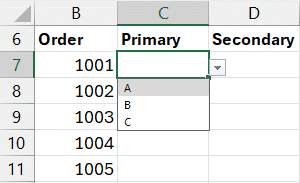
The order list, including the columns for our primary and secondary drop downs, looks something like this:

We want a pair of drop downs for each row.

Let’s start with the primary drop down.

First, we’ll create a range that will include a unique list of the values found in the Primary column of the choices table (Table1). Although we could simply type the values in a range, we’ll use a formula so that the list is dynamic … meaning any new rows added to the choices table (Table1) will automatically be included.

We’ll write this formula on a new worksheet, or really anywhere within the workbook we’d like:

=UNIQUE(Table1[Primary])

We hit Enter and bam:

This formula creates a unique list of the values in the table’s Primary column, and will automatically update it results to include any new rows added in the future. The results returned will provide the list of choices in our primary drop down.

Our next step will be to define a friendly name that we can use to reference this dynamic list of primary drop down choices. For this illustration, we’ll name the dynamic range dd_primary (for primary drop down). To define this name:

Go to Formulas > Name Manager > New.

In the Name field of the resulting dialog, name it dd_primary (or any other preferred name; this specific name isn’t important to Excel)

In the Refers to field, start with an equal sign to reference the formula cell $B$8 and use the spill operator # like this:

Notes: be sure to use an absolute cell reference (with the dollar signs) and be sure to add the spill operator # so that future options will be included. You can use any preferred name besides dd_primary … just avoid spaces and funky characters. The name I used above isn’t significant to Excel.

With our name set up, we can now create our drop downs.

Select the range where you want the primary drop downs:

Go to Data > Data Validation.

Allow a list and set the source to =dd_primary (or whatever name you may have used instead):

Now as you select any cell in the selected range, you’ll see a drop down and can select a choice:

Our final step is to create the secondary drop downs.

Exercise 3: Secondary Drop Downs

We will once again create a new name. This time, we’ll call our name dd_secondary (but again, you can use a different name if preferred).

Before we jump into the Name Manager to create the new name, we’ll want to understand what the name will refer to. We want to point it to the range that represents valid secondary choices based on the selected primary choice. So, assuming we select A in the primary drop down like this:

We want the name to point to the valid secondary cells in the choices table:

To define this range, we’ll use two XLOOKUP functions that locate the first valid choice and the last valid choice based on the selected primary value. In other words, if we select A as the primary choice, the first XLOOKUP function will locate the first A row while the second XLOOKUP function will locate the last A row.

You are already familiar with the range reference operator, the colon :. It is how we define a range. We typically define a range by identifying the upper-left cell in the range, then using the colon, and then identifying the lower-right cell in the range. For example, a classic range may look like this:

=A1:A10

This refers to the range of cells between A1 and A10 inclusive.

Well, in addition to using cells on both sides of the reference operator, we can use XLOOKUP. For example, we could create a similar range like this (for simplicity, I left out the function arguments):

=XLOOKUP:XLOOKUP

The first XLOOKUP function defines the first cell in the range, and the second XLOOKUP defines the last cell in the range.

So, our goal will be to write two XLOOUP functions … one that returns the first row for the selected primary value and one that returns the last row. Then, we’ll use them on either side of the range operator.

Let’s write the following formula into D7 (broken down into three rows for clarity):

=XLOOKUP(C7,Table1[Primary],Table1[Secondary])
:
XLOOKUP(C7,Table1[Primary],Table1[Secondary],,,-1)

This constructs a range using two XLOOKUP functions:

1. First XLOOKUP: Finds the first value in the Table1[Primary] column that matches the value in cell C7, and it returns a reference to the corresponding cell in the Table1[Secondary] column.
2. Second XLOOKUP: Finds the last value in the Table1[Primary] column that matches the value in C7. It essentially performs the same lookup, but searches in reverse order (last to first), thanks to the -1 value for the search_mode.

The colon (:) creates a range reference to the cells between these two lookup results, inclusive.

If you aren’t familiar with XLOOKUP, here is a basic summary:

XLOOKUP(C7, Table1[Primary], Table1[Secondary])

• C7: This is the value you’re looking for.
• Table1[Primary]: This is the column where Excel will search for the value in C7.
• Table1[Secondary]: Once Excel finds a match, it returns the corresponding reference/value from this column.

In simple terms, it looks for the value in C7 in the Table1[Primary] column and returns the corresponding reference/value from the Table1[Secondary] column.

After writing the formula in D7, we hit Enter and bam:

As you can see, it returns the range of targeted cells in the Secondary column in the choices table:

So, since we wrote this formula into the same cell that we want our secondary drop down, we can simply copy/paste the formula into the Name Manager.

So, begin by selecting the formula text and doing a standard copy.

Then, go to Formulas > Name Manager > New.

Name it dd_secondary.

Paste the formula (including the equal sign =) into the “Refers to” field:

After we have pasted this formula for the defined name, we can delete the formula from the worksheet cell D7.

And once again, we’ll use our defined name as the source for our drop down.

Select the range for the secondary drop down:

Go to Data > Data Validation

Allow a list and set the source to =dd_secondary

Now, once you have make a selection from the primary drop down, the resulting secondary drop down will reveal the corresponding choices:

Change the primary choice and the corresponding secondary choices will be displayed.

So, that is one way to create dependent drop downs for many rows.

Optional: Notify Users of Invalid Choices

When the primary drop down changes, previously selected secondary options may no longer be valid. Excel doesn’t automatically clear these values, but you can use Conditional Formatting to alert users. To do so, select the secondary drop down range (D7:D11 in this example) and:

1. Set Up Conditional Formatting:
   • Go to Home > Conditional Formatting > New Rule.
   • Use a formula: =COUNTIFS(Table1[Primary], C5, Table1[Secondary], D5) = 0
   • Format the cell (e.g., red fill) to indicate an invalid choice.
2. Exclude Empty Cells:
   • Add another rule for blanks
   • Set no formatting.
   • Ensure this rule has “Stop if True” enabled.

Setting up conditional formatting simply communicates to the user that the change of a primary choice created an invalid cell value in the secondary column, like this:

By following these steps, you’ll have a robust, scalable solution for dependent drop downs in Excel. If you have any questions or additional tips, feel free to share them in the comments below!

Sample File

Download a sample file to follow along and explore the formulas.

Frequently Asked Questions

1. Can I use this method without sorting the table?

Sorting ensures XLOOKUP captures the correct range. If the table is not sorted by the Primary column, unexpected choices will appear in the secondary drop down.

2. What if I want to apply this to multiple rows?

This setup is inherently row-based. Use relative references to replicate drop downs across rows.

3. Can I handle more than two levels of drop downs?

Yes. Use this same technique for additional columns. Once again, be sure to sort the choices table accordingly.

4. Why is my drop down showing incorrect or blank results?

Double-check the XLOOKUP formula and ensure the named ranges are set up correctly.