Conditionally Format Input Cells

Hello, Excel enthusiasts! Today, we’re diving into a neat trick: automatically formatting input cells based on whether they meet specific criteria. The goal? Identify and format cells where the first digit of the input is a “4.” But, you can apply this same technique to other criteria.

By the end of this post, you’ll have a clear understanding of how to apply conditional formatting, using a simple formula to automate this process. Let’s break it down into three easy steps!

Video

Step-by-step Tutorial

Let’s walk through the details using several exercises to illustrate.

Exercise 1: Manual Approach

Let’s say we have a list of orders like this:

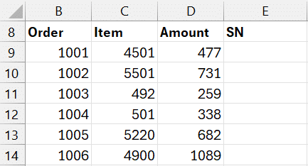
When the Item begins with a 4, we need to enter the serial number in the SN column. To make it easy for the data entry, we’d like to format the SN cells so it is obvious which ones require input, like this:

One option is to manually format the cells. But, manually formatting cells can be tedious, especially when dealing with large datasets. Imagine reviewing hundreds or thousands of item numbers, checking for a specific condition, and formatting cells one by one.

Instead, we can use conditional formatting to save time and ensure accuracy. But since we are formatting a cell based on the value in another, we’ll need to first understand how to write a formula that returns TRUE when our condition is met (in this case, when the Item starts with 4).

Exercise 2: Create a Formula to Identify Cells

In this illustration, the condition is that the item number must start with the digit “4.” When it does, we want Excel to automatically format the SN cell to indicate it needs a serial number.

The first step is crafting a formula that checks whether the first character of a cell is “4.” For this, we’ll use the LEFT function, which extracts characters from the start of a text string.

Here’s the formula that we could write in E9:

=LEFT(C9)="4"

How it Works

1. LEFT(C9) pulls the first character from the cell.
2. The = "4" part checks if the extracted character is “4.” Note that we surround the 4 in quotes because the LEFT function returns a text string. So, the text string returned by the LEFT function would not be equal to the numeric equivalent 4. By enclosing the 4 in quotes, we ensure the comparison is between two text strings.
3. The formula returns TRUE if the first character is “4” and FALSE otherwise.

For example, this would be the formula result based on the given Item Number:

Item Number	Formula Result
40123	TRUE
35289	FALSE
41234	TRUE

Now that we understand how to write a formula that returns TRUE when the first character of the Item begins with 4, we can proceed to create a conditional formatting formula.

Exercise 3: Conditional Formatting Formula

We’ll use a similar formula to create a conditional formatting rule. Follow these steps:

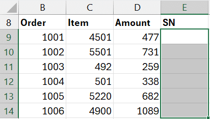
Select the range of cells to format (e.g., E9:E14):

Go to the Home tab, click Conditional Formatting, and select New Rule.

In the resulting New Formatting Rule dialog, choose “Use a formula to determine which cells to format.”

Enter the formula:

=LEFT(C9)="4"

⚠️ Ensure that the cell reference (e.g., C9) is a relative reference (no dollar signs), relative to the Active cell (in this screenshot, the Active cell is E9).

Click Format to define the desired format and click OK.

Once applied, Excel will scan the selected range and automatically format any cell where the item number starts with “4.”

This visual cue helps you quickly identify which cells need additional action, like entering a serial number.

Note: you can customize the Conditional Formatting Formula as desired … the main keys are (a) it should return a TRUE value when you want the formatting applied and (b) use relative references (no dollar signs) relative to the Active cell when using this technique.

Wrapping Up

Conditional formatting is a powerful tool that makes your spreadsheets more intuitive and efficient. By using conditional formatting formulas, we can quickly identify specific conditions—like item numbers starting with “4”—and apply formatting to highlight them.

Using conditional formatting with a formula has several advantages:

• Saves time: No need for manual cell-by-cell formatting.
• Dynamic: Automatically updates as data changes.
• Error-free: Ensures consistent application of rules across the dataset.

Have questions about this technique or suggestions for other Excel topics? Let us know in the comments below. We’d love to hear from you!

Sample File

FAQs

1. Can I use this method for other conditions?

Absolutely! Just be sure the conditional formatting formula returns TRUE when you want the formatting applied.

2. Can I apply multiple conditional formatting rules?

Yes, Excel allows you to layer multiple rules. For example, you could format cells starting with “4” in yellow and cells starting with “3” in blue by applying two formatting rules the the same range.

3. What if I want to format entire rows, not just cells?

Begin by selecting the range you want to conditional formatting (it would span many columns). Use the same basic formula, but adjust the cell reference to use an absolute column/relative row reference like this: $C9.

4. Does conditional formatting slow down Excel?

In practice, I have not noticed any performance hit with conditional formatting.

5. How do I clear conditional formatting?

Go to Home > Conditional Formatting > Clear Rules, and choose whether to clear rules from the selected cells or the entire sheet.

6. What about looking at the first two characters?

By default, the LEFT function extracts the first character from the cell. However, there is an optional argument that enables us to define the number of characters to extract. To extract the first two characters from C9, we would use LEFT(C9,2). To get the first 3, we use LEFT(C9,3) and so on.