Return the Sum of Two or More Columns with VLOOKUP
If you have ever wished that the VLOOKUP function could return the sum of two or more related columns, this trick will get you there.
Objective
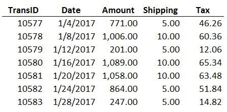
Before we get into the details, let’s be clear about our objective. We have some transactions that were exported from our accounting system as shown below.
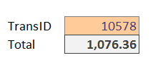
We would like to write a formula that will look up any given TransID and return the sum of three columns, Amount, Shipping, and Tax. This is illustrated in the screenshot below, where we enter a TransID such as 10578 and Excel computes the Total (1,076.36 = 1,006 + 10 + 60.36).
Since this is essentially a lookup task, our first instinct is to use VLOOKUP. However, we know that VLOOKUP can only return one related value, not the sum of multiple related values.
One common workaround is to add a helper column to the data that sums the three columns and then use a VLOOKUP to return the value from the new helper column. However, whenever possible in practice, we prefer to work with the data as it comes so that the workbook is easy to update in future periods.
Another common workaround is to write a formula that adds up three VLOOKUP functions, such as the following.
=VLOOKUP(...) + VLOOKUP(...) + VLOOKUP(...)
However, such a formula can be difficult to update and maintain over time since any change to the arguments need to be made three times instead of once. The good news is that we can wrap a SUMPRODUCT function around a single VLOOKUP function. Let’s get started.
SUMPRODUCT
When the SUMPRODUCT has a single argument, it behaves much like the SUM function because it simply returns the sum of the values. When the SUMPRODUCT has multiple arguments, it returns the sum of the product of its arguments. To accomplish our objective, we will use the SUMPRODUCT to return the sum of the values in a single argument.
Basically, we will wrap a SUMPRODUCT function around a VLOOKUP function that returns an array of values, specifically, the related values from multiple columns. The SUMPRODUCT will sum the values in the array returned by the VLOOKUP function. How do we convince the VLOOKUP function to return an array of values? That brings us to our next discussion.
Technical Note: we need to use SUMPRODUCT instead of SUM because the SUMPRODUCT function is designed to work with arrays and will thus return the sum of the array returned by the VLOOKUP function. The SUM function would return the sum of the first array element only. However, you could use the SUM function and then array-enter it with Control+Shift+Enter if preferred.
Array of Values
We can ask the VLOOKUP function to return an array of values by enclosing the third argument in curly braces {}. This causes the VLOOKUP function to actually return an array that contains multiple elements. For example, if we wanted the VLOOKUP function to return the values from the 3rd, 4th, and 5th columns to an array with three elements, we could use the following formula.
=VLOOKUP(C6,B12:F18,{3,4,5},0)
Where:
- C6 is the lookup value
- B12:F18 is the lookup range
- {3,4,5} are the column numbers that have the values we want returned, enclosed in curly braces to create the array of values
- 0 tells VLOOKUP to use exact match logic
This VLOOKUP function actually returns an array of values, and the array elements are 1006, 10, and 60.36. If you enter it into a single cell and press Enter, Excel will display only the first element. But, we don’t want to display the first element, we want to compute the sum of all array elements. So, let’s put it all together and bring it home.
Technical note: you can confirm the VLOOKUP returns an array of values by array-entering the formula into three cells across at once (Ctrl+Shift+Enter). Excel will display the three array elements in the three cells.
SUMPRODUCT and VLOOKUP
Now that we understand that using the curly braces causes VLOOKUP to return an array of values, let’s add up the values in the returned array with the SUMPRODUCT function.
Here is a screenshot of our workbook.
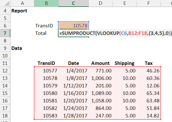
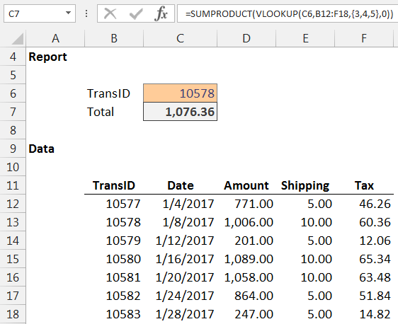
The formula in C7 follows.
=SUMPRODUCT(VLOOKUP(C6,B12:F18,{3,4,5},0))
The SUMPRODUCT function returns the sum of the array elements returned by the VLOOKUP function. This is essentially the same as SUMPRODUCT({1006, 10, 60.36}), which returns 1076.36.
When we press Enter, we confirm that it works as expected…yes!
Note: there is no need to array-enter this formula by using Control-Shift-Enter.
And that my friend is one way to return the sum of two or more columns with VLOOKUP. If you have another approach, please share by posting a comment below…thanks!
Additional Resources
Excel is not what it used to be.
You need the Excel Proficiency Roadmap now. Includes 6 steps for a successful journey, 3 things to avoid, and weekly Excel tips.
Want to learn Excel?
Our training programs start at $29 and will help you learn Excel quickly.
That’s really clever! How did you run across the option of putting an array of columns into the VLOOKUP function?
Joe,
That technique came from a participant in a discussion during one of my Excel sessions…pretty cool!
There is so much to learn about Excel…I wish I had discovered that trick years ago 🙂
Thanks
Jeff
Excellent – thank you. Is there any way to replace the {3,4,5} part with a name? Like can I name a group of columns and reference them that way? Not finding anything about naming an array.
Hey Jon,
You can create a named formula, as in ={3,4,5}, and use that instead:)
Let me know if you need anymore help!
Kurt LeBlanc
Jeff, this is a really cool solution.
More to the point – you explain it clearly and succinctly in a way that is not only easy to follow, but helps to ‘stick’ it in the brain.
You’re clearly a gifted teacher.
Nick
Thanks 🙂
Will this similarly work with hlookup?
Correct! It works because SUMIFS() works horizontally as well as vertically.
Thanks for the useful information.. I would like to add multiple values which are in the same column (unlike the example here where the addition is along the same row)…How do I do that. Can you please suggest.?
Hey Srinkanth!
Absolutely, with HLOOKUP:) It is exactly the same logic fortunately, just with nth row as the third argument instead of column. If you transpose the table in the sample file and adjust the lookup formula to HLOOKUP(), you can see hat even the array works as expected:)
Let me know if you need any help with the setup,
Kurt LeBlanc
Hi Kurt,
My table area is A1:K30. My Lookup value matches with H1. And I want to add from H10 to H28. Instead of writing all the row numbers from 10 to 28 withing HLookup [ like – hlookup{10,11,12,13,…….,26,27,28} ] is there any other options?
I understand now:)
Unfortunately, you have to enter each of the individual numbers in the array…or you can create a named formula that refers to the array, and use that in your lookup.
Let me know if that is clear
Kurt LeBlanc
This post is to subscribe to follow-up emails (meant to do that earlier, but forgot)
Great…thanks!
Thanks this is a great post. However, what’s missing is the solution that sums up multiple values in one column. All the values I want to sum up are not in multiple columns but in the same column. How do I make this work? Thanks in advance
Hi Sam! Summing values in a single column is discussed in this post:
https://www.excel-university.com/multiple-condition-summing-in-excel-with-sumifs/
Hope it helps!
Thanks
Jeff
Good day,
I really benefit from this – Thank you!!
Just a question I have a vlookup table A:Q3229 and needs to sum the months from Jan to June (depending on the month). Please see my formula below:
{=IFERROR(SUM(VLOOKUP(E18,budget!A:Q,{5,6,7,8,9,10},0)),””)} this formula is working perfectly – however is there a way if you change the month in the input sheet that it can add a column (Jan to July) to add instead of adding column 11 to my formula?
I would like to sent the sheet out to individuals to fill in and they won’t be able to change the formula.
I’d probably suggest using SUMIFS instead of VLOOKUP, which supports the use of comparison operators (such as > and <) in the criteria arguments. I've written a bunch of posts on SUMIFS if you haven't used it before: https://www.excel-university.com/tag/sumifs/
Hope it helps,
Jeff
Hello,
If I where to have multiple “lookup values” in a table and I´d like the sum of all ID “a”
ID
a 3 4 1
b 4 5 2
c 6 1 5
a 7 2 0
d 1 1 9
a 0 1 7
ID a
Total = 3+4+1+7+2+0+0+1+7
How could I achive this? using the formula it only gives me: 3+4+1
You could probably accomplish that with SUMIFS, which returns the sum of all matching rows. I have a post that discusses this function:
https://www.excel-university.com/multiple-condition-summing-in-excel-with-sumifs/
Hope it helps!
Thanks
Jeff
Very useful post for Excel users. Thanks a lot for this post.
Hello Jeff,
Thank you for the incredibly useful article!
I have a unique situation and I was wondering if you could help me out. I have monthly income statement data (from Jan-Dec) in one tab and an output page on another tab. On the output page, I have two cells – beginning month and ending month; which reflects the performance period I want to look at. I.e. if I wanted to see the performance for January thru June, I would enter 1 and 6 in the respective cells.
My question is: is there any way I can sum the revenues (as an example) for the different columns by using a combination of vlookup and sumproduct? I can’t use the technique you described because the column numbers here are hard-coded whereas I am trying to make my output page more dynamic so I don’t have to go in and change the formula every time.
Thank you so much for your help in advance.
Many thanks, but could I simply things;
=SUMPRODUCT(($G$5:$I$11)*($L$4=$E$5:$E$11))) = 1076.36
simply using sumproduct without a lookup function will work as above where cell L4 = 10578
There are many ways, just thought I would add another!
Kind regards
Nice … thanks!
very good !.
Hi Jeff,
Do you know of a way this could be expanded so that the formula is able to find more than one “hit” for the lookup value?
I have a table of data where the lookup value could appear up to three times in column B. The formula would then have to be able to sum values from, for example, cell D12, E12, F13 &/or F14.
I think it would be either Sumproduct or Index Match Match but I have tried numerous different formulas with no luck.
Hopefully this makes sense and thank you in advance for any help you can offer.
Kind regards
Matt
do you have formula for the vlookup with match function and sum multiple columns of match function?
I have a multi sheet spread sheet keeping track of job hours. I have used VLOOKUP in succession to sum all the hours on multiple sheets and it works great… Until it gets to a sheet that does not contain the lookup value. I have searched all over for my issue, and VLOOKUP may be the incorrect solution. I was wondering if I could rattle anyone’s brain to make this work.
I have 1 excel document with 52 tabs. Each tab is a work week starting from January so WW1 is all the hours for sed jobs the first week of January. “joes house 2 hours ; mikes house 3 hours”… I then have created all 52weeks as tabs… WW2, WW3 etc… Until WW52.
This is the function I made to add hours together…
=SUM(VLOOKUP(O30,’WW29′!$A$7:$M$110,{13},FALSE),VLOOKUP(O30,’WW30′!$A$7:$M$110,{13},FALSE),VLOOKUP(O30,’WW31′!$A$7:$M$110,{13},FALSE))
And it works great. But when that job is finished it is not on (for example WW32 tab), I get the #N/A error. So for example, as the previous one works great when I expand the formula to cover the next sheet (“WW32” EXAMPLE OF NEXT PAGE WIOTHOUT LOOKUP VALUE)
=SUM(VLOOKUP(O30,’WW29′!$A$7:$M$110,{13},FALSE),VLOOKUP(O30,’WW30′!$A$7:$M$110,{13},FALSE),VLOOKUP(O30,’WW31′!$A$7:$M$110,{13},FALSE),VLOOKUP(O30,’WW32′!$A$7:$M$110,{13},FALSE))
I get the #N/A error because the job is not listed on WW32. But I may need to add hours to a certain job on WW45 due to say a change order. Therefore I would like to sum all 52 weeks and have a total sheet at the end. Is there a way to make VLOOKUP skip a sheet that does not have the referenced value and continue summing it till the end? I apologize, this may be as clear as mud but I will clarify anything if need be. I have also tried IFERROR. You can set IFERROR to return text or even blanks, but does not seem to cover summing. I’m looking for how to SUM multiple sheets when some of the sheets do not contain the lookup value. When using IFERROR function, instead of RETURNING #N/A it just returns “YOU’VE ENTERERED TOO MANY ARGUMENTS FOR THIS FUNCTION”…
=IFERROR(VLOOKUP(O30,’WW29′!$A$7:$M$110,{13},FALSE),VLOOKUP(O30,’WW30′!$A$7:$M$110,{13},FALSE),VLOOKUP(O30,’WW31′!$A$7:$M$110,{13},FALSE),VLOOKUP(O30,’WW32′!$A$7:$M$110,{13},FALSE),””)And that’s just 3 sheets.
Any help would be greatly appreciated.
P.S. I have tried with CTRL+SHIFT+ENTER as well to no avail.
HOW TO CONVERT THE COLUMN APPROACH IN TO DYNAMIC
I am trying to use the IF(ISNA(sumproduct(VLOOKUP($A2,’Apr 2023 DX’!$A:$J,{4,5,6,7,8,9,10},0)))) but it doesn’t want to work. Any suggestions. I am trying to have it return an empty cell if “N/A” is the answer.