Power Query and Zip Code Formatting

Power Query is an amazing tool, and I love learning about it. In the Power Query Editor, as you click the command icons, Excel is actually writing M code behind the scenes. M code has many more functions than are available in the ribbon. So, the thing to keep in mind is that if you are trying to accomplish something, and don’t see a command icon, dig into the functions because there is a good chance you’ll find something helpful. In this post, I’ll illustrate this by adding leading zeros to a zip code.

Objective

Before we get too far, let’s confirm our goal here. Let’s say we are using Power Query to import and clean some data. We are able to accomplish everything we need by clicking command icons, and we are almost done … except for one little thing. We can’t seem to find a command that will format the zip codes with leading zeros.

We search through the Query Editor ribbon, click all the icons, right-click everyplace we can think of, and nothing. Now, this is the point of this post. Not all PQ functions are available in the ribbon. So, we’ll need to roll up our sleeves and dig into the M functions. Ready? Me too!

Details

To accomplish this task, we’ll perform these basic steps:

• Get the data into PQ
• Zips with leading zero
• Send results to Excel

Let’s get to it.

Note: The steps below are presented with Excel for Windows 2016. If you are using a different version of Excel, please note that the features presented may not be available or you may need to download and install the Power Query Add-in.

Get the data into PQ

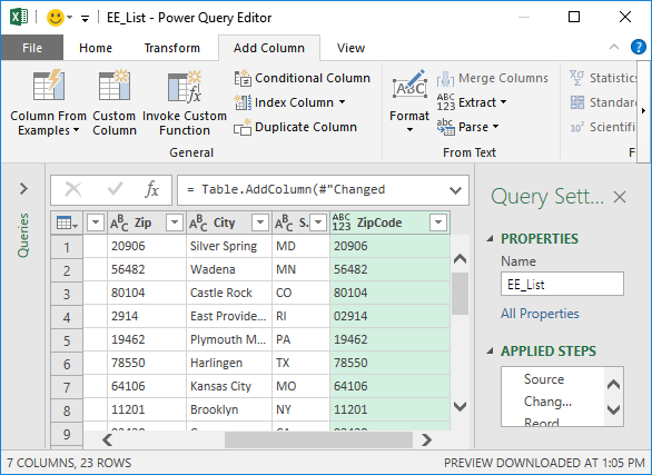
First, we need to get the data into the Power Query editor. This is done by selecting any cell in the Table and clicking Data > From Table/Range. Excel then displays the Power Query Editor, as shown below.

With our data in PQ, it is time for the next step.

Zips with leading zero

Now, we’d like our Zip column to display a leading zero when needed. For example, instead of 2914 we want 02914. As with just about anything, there are multiple ways to accomplish this task.

If you are like me, your first instinct is to start exploring the command icons. As we click through them, searching the Format command, Fill, Replace Values, Data Type, Extract, Column from Examples, Standard, and more, we can’t seem to find anything that will work.

One option would be to do a Conditional Column, where we try to determine the length of the zip and concatenate a leading zero if the length is 4. Another possibility is to send the results to Excel as they are, and then handle the formatting in Excel with a custom 00000 format. And yet another possibility is to use a built-in M function that is designed exactly for this purpose. Let’s give that option a try.

First, we need to change the data type of the Zip column from a number to a text. To do this, we select the Zip column and then click Transform > Data Type > Text.

Second, we need to create a new custom column by clicking Add Column > Custom Column. This opens the Custom Dialog, as shown below.

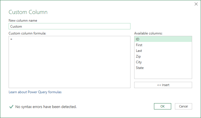
Now, at this point, we have no idea about which M function can help, or, if there even is one. So, we need to do a bit of research. We click the Learn about Power Query formulas link in the Custom Column dialog and up pops the help page, as shown below.

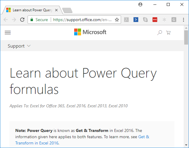
This page provides a basic overview, but, there is a key link if you scroll down a bit called Power Query formula categories as shown below.

Click this link and you find the Power Query M function reference page, shown below.

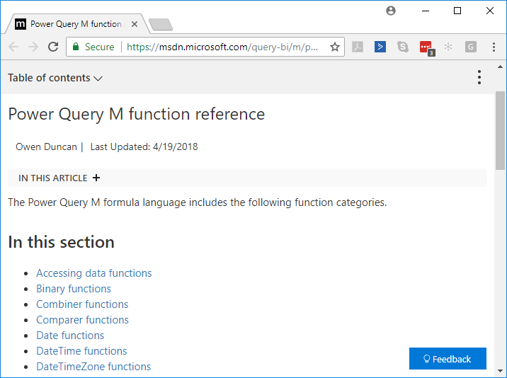
It displays the categories of M functions, and would be a good page to bookmark for quick reference. In this case, we are looking for a function that operates on our text zip code, so we click the Text functions link. We can scroll down the page, viewing each function and reading a brief description. As we scroll down, we see the Text.PadStart function, which, based on its description, returns a text value padded at the beginning. That sounds like what we want to do, so we click the function link.

Now, we see the details of the function, and can learn about its arguments. which in this case, are text, length, and pad. Once we have a basic understanding of the function and arguments, we need to give it a try. So, we head back to the Custom Column dialog, and write the function and define the arguments. It is important to note that functions are case-sensitive in Power Query. This is different from Excel function, which are case-insensitive.

So, in the Custom Column dialog, we enter our desired New column name, ZipCode. Then, we start writing the formula by typing =Text.PadStart( and are sure to use the exact upper case and lower case letters from the function details page.

Our first argument is text, which is the zip code column. So, we double-click Zip from the Available columns list box and see that Excel enters [Zip] with square brackets. Then we type a comma and we’re ready for the next argument.

The next argument is length, and so we enter 5 to force all zip codes to 5 characters. We enter a comma, and are ready for our last argument.

The final argument is pad, and since our zip code is a text string we need to enter a text value enclosed in quotes. So we enter “0” and close the function as follows:

=Text.PadStart([Zip],5,"0")

The updated Custom Column dialog is shown below.

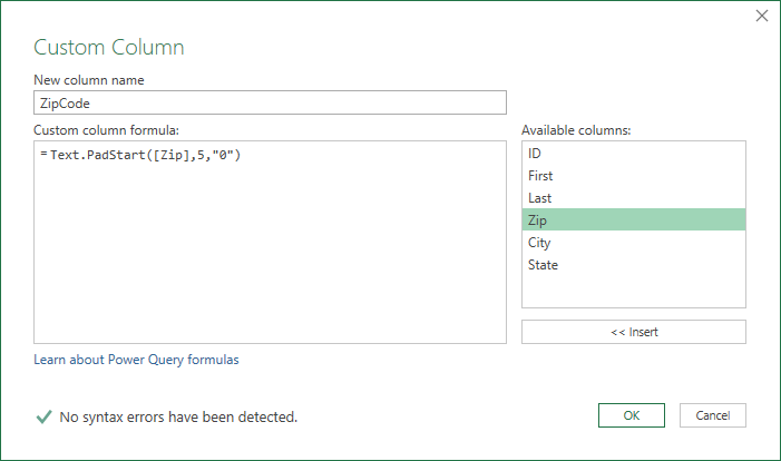
In the bottom of the dialog, we see a green check that no syntax errors have been detected, so we click OK.

Yes …  it works, as shown below.

Note: Thanks to Mynda who wrote about this function and showed how to enclose the text argument in quotes! If you’d like to learn more about Power Query from Mynda, check out her Power Query for Excel course … which is available for CPE credit if you need it.

With our new ZipCode column, we can now remove the original Zip column by selecting it and then clicking the Remove Columns command.

M Code Note

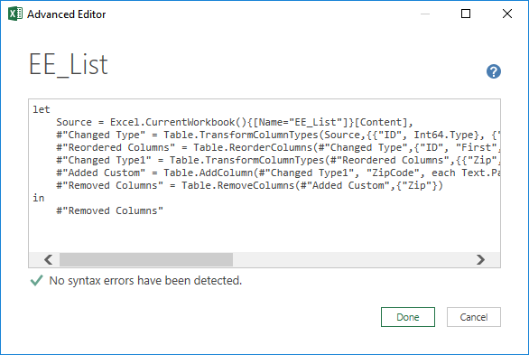
Now, here is an interesting note. Basically, the command icons we click in the Power Query Editor ribbon create M code. For example, click on View > Advanced Editor to see the M code generated, as shown below.

And, a really handy option if you are trying to learn about M code, is to toggle on the display of the formula bar by checking the View > Formula Bar checkbox. This allows you to see the M code generated as you work, and, you can even make edits there.

In any event, our zip code column is looking good, so it is time to send our results back to Excel.

Send results to Excel

Click Close & Load, and bam, the results appear in our worksheet as shown below.

And, that my friend, is how to discover M functions that can really help you leverage this amazing tool!

If you have any other M functions you find useful, please share by posting a comment below.

Sample file

• Zip.xlsx